

2.3 The Born–Oppenheimer Approximation and Its Breakdown …
37
Here and in the following, a subscript added to a bracket expression indicates the
integration variables, when needed for clarity. Moreover, |ϕ(r; R)|
2 (which is given
by the ratio |ψ|
2
/ |χ |
2 ) represents the probability density to find the electrons in r,
once the nuclei have been fixed in the positions R: it is then a conditional probability.
Note that ϕ(r; R) is by no means a nuclear wavefunction, but of course it depends
parametrically on the nuclear coordinates R.
The Born–Oppenheimer (BO) approximation consists in assuming specific forms
of the electronic and the nuclear wavefunctions, consistent with the above requirements (2.54) and (2.55). In particular, the electronic wavefunctions are defined as
the eigenfunctions of the electronic Hamiltonian ˆ
H el :
ˆ
H el = ˆ
H mol − ˆ
T n = ˆ
T e + V el + ˆ
V s
(2.56)
ˆ
H el (r, R)ϕ k (r; R) = U k (R)ϕ k (r; R)
(2.57)
where U k (R) is the electronic energy and k is the index enumerating the eigenstates.
The energies and wavefunctions so defined are called “adiabatic.” Since ˆ
H el is Hermitian, we can require ϕ k |ϕ l r = δ kl . Given that the electronic motion is much
faster than the nuclear one, it is assumed that the electronic energy U k plays the
role of potential energy surface for the nuclear motion. In particular, the nuclear
wavefunctions belonging to the electronic potential energy surface (PES) U k (R) are
determined as eigenfunctions of the nuclear Hamiltonian ˆ
H
(k)
n
ˆ
H
(k)
n = ˆ
T n + U k
(2.58)
ˆ
H
(k)
n (R)χ kv (R) = E kv χ kv (R)
(2.59)
where v is the index enumerating the nuclear (vibrational) states and E kv is the total
energy. In the above, R represents the 3N n Cartesian coordinates of the nuclei, or
the 3N n − 6 internal coordinates, after separation of translations and rotations. In
the latter case M α have to be replaced by the relevant reduced masses in ˆ
T n , and
we assume anyway that the internal coordinates are fixed and orthogonal (i.e., they
verify Eqs. (2.41) and (2.49)), so that ˆ
T n keeps the diagonal form of Eq. (2.33).
Within the BO approximation, a given eigenstate of the molecular Hamiltonian is
equal to the “vibronic” product ϕ k (r; R)χ kv (R), and the corresponding energy is E kv
(see Eqs. (2.57) and (2.59)). To judge about the quality of the BO approximation, let
us evaluate the matrix elements of ˆ
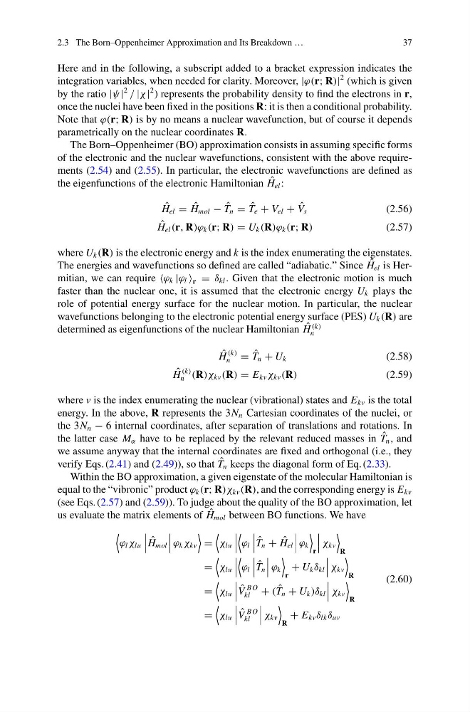
H mol between BO functions. We have
ϕ l χ lu
ˆ
H mol
ϕ k χ kv
=
χ lu
ϕ l
ˆ
T n + ˆ
H el
ϕ k
r
χ kv
R
=
χ lu
ϕ l
ˆ
T n
ϕ k
r
+ U k δ kl
χ kv
R
=
χ lu
ˆ
V
B O
kl + ( ˆ
T n + U k )δ kl
χ kv
R
=
χ lu
ˆ
V
B O
kl
χ kv
R
+ E kv δ lk δ uv
(2.60)
37
Here and in the following, a subscript added to a bracket expression indicates the
integration variables, when needed for clarity. Moreover, |ϕ(r; R)|
2 (which is given
by the ratio |ψ|
2
/ |χ |
2 ) represents the probability density to find the electrons in r,
once the nuclei have been fixed in the positions R: it is then a conditional probability.
Note that ϕ(r; R) is by no means a nuclear wavefunction, but of course it depends
parametrically on the nuclear coordinates R.
The Born–Oppenheimer (BO) approximation consists in assuming specific forms
of the electronic and the nuclear wavefunctions, consistent with the above requirements (2.54) and (2.55). In particular, the electronic wavefunctions are defined as
the eigenfunctions of the electronic Hamiltonian ˆ
H el :
ˆ
H el = ˆ
H mol − ˆ
T n = ˆ
T e + V el + ˆ
V s
(2.56)
ˆ
H el (r, R)ϕ k (r; R) = U k (R)ϕ k (r; R)
(2.57)
where U k (R) is the electronic energy and k is the index enumerating the eigenstates.
The energies and wavefunctions so defined are called “adiabatic.” Since ˆ
H el is Hermitian, we can require ϕ k |ϕ l r = δ kl . Given that the electronic motion is much
faster than the nuclear one, it is assumed that the electronic energy U k plays the
role of potential energy surface for the nuclear motion. In particular, the nuclear
wavefunctions belonging to the electronic potential energy surface (PES) U k (R) are
determined as eigenfunctions of the nuclear Hamiltonian ˆ
H
(k)
n
ˆ
H
(k)
n = ˆ
T n + U k
(2.58)
ˆ
H
(k)
n (R)χ kv (R) = E kv χ kv (R)
(2.59)
where v is the index enumerating the nuclear (vibrational) states and E kv is the total
energy. In the above, R represents the 3N n Cartesian coordinates of the nuclei, or
the 3N n − 6 internal coordinates, after separation of translations and rotations. In
the latter case M α have to be replaced by the relevant reduced masses in ˆ
T n , and
we assume anyway that the internal coordinates are fixed and orthogonal (i.e., they
verify Eqs. (2.41) and (2.49)), so that ˆ
T n keeps the diagonal form of Eq. (2.33).
Within the BO approximation, a given eigenstate of the molecular Hamiltonian is
equal to the “vibronic” product ϕ k (r; R)χ kv (R), and the corresponding energy is E kv
(see Eqs. (2.57) and (2.59)). To judge about the quality of the BO approximation, let
us evaluate the matrix elements of ˆ
H mol between BO functions. We have
ϕ l χ lu
ˆ
H mol
ϕ k χ kv
=
χ lu
ϕ l
ˆ
T n + ˆ
H el
ϕ k
r
χ kv
R
=
χ lu
ϕ l
ˆ
T n
ϕ k
r
+ U k δ kl
χ kv
R
=
χ lu
ˆ
V
B O
kl + ( ˆ
T n + U k )δ kl
χ kv
R
=
χ lu
ˆ
V
B O
kl
χ kv
R
+ E kv δ lk δ uv
(2.60)