

Appendix D
Two-State Eigenvector Problem
Although this problem is trivial, it is convenient to write out its solution that is
referred to more than once in this book, in order to use the same formulation in
all cases. By doing so, we shall remove some arbitrariness which is intrinsic of
eigenvector problems (signs or phase factors and ordering of eigenvectors), by setting
our conventional choices.
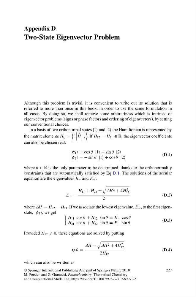
In a basis of two orthonormal states |1 and |2 the Hamiltonian is represented by
the matrix elements H i j =
i
ˆ
H
j
. If H 12 = H 21 ∈ R, the eigenvector coefficients
can also be chosen real:
|ψ 1 = cos θ |1 + sin θ |2
|ψ 2 = − sin θ |1 + cos θ |2
(D.1)
where θ ∈ R is the only parameter to be determined, thanks to the orthonormality
constraints that are automatically satisfied by Eq. D.1. The solutions of the secular
equation are the eigenvalues E − and E + :
E ± =
H 11 + H 22 ±
ΔH 2 + 4H
2
12
2
(D.2)
where ΔH = H 22 − H 11 . If we associate the lowest eigenvalue, E − , to the first eigenstate, |ψ 1 , we get
H 11 cos θ + H 12 sin θ = E − cos θ
H 21 cos θ + H 22 sin θ = E − sin θ
(D.3)
Provided H 12 = 0, these equations are solved by putting
tg θ =
ΔH −
ΔH 2 + 4H
2
12
2H 12
(D.4)
which can also be written as
© Springer International Publishing AG, part of Springer Nature 2018
M. Persico and G. Granucci, Photochemistry, Theoretical Chemistry
and Computational Modelling, https://doi.org/10.1007/978-3-319-89972-5
227
Two-State Eigenvector Problem
Although this problem is trivial, it is convenient to write out its solution that is
referred to more than once in this book, in order to use the same formulation in
all cases. By doing so, we shall remove some arbitrariness which is intrinsic of
eigenvector problems (signs or phase factors and ordering of eigenvectors), by setting
our conventional choices.
In a basis of two orthonormal states |1 and |2 the Hamiltonian is represented by
the matrix elements H i j =
i
ˆ
H
j
. If H 12 = H 21 ∈ R, the eigenvector coefficients
can also be chosen real:
|ψ 1 = cos θ |1 + sin θ |2
|ψ 2 = − sin θ |1 + cos θ |2
(D.1)
where θ ∈ R is the only parameter to be determined, thanks to the orthonormality
constraints that are automatically satisfied by Eq. D.1. The solutions of the secular
equation are the eigenvalues E − and E + :
E ± =
H 11 + H 22 ±
ΔH 2 + 4H
2
12
2
(D.2)
where ΔH = H 22 − H 11 . If we associate the lowest eigenvalue, E − , to the first eigenstate, |ψ 1 , we get
H 11 cos θ + H 12 sin θ = E − cos θ
H 21 cos θ + H 22 sin θ = E − sin θ
(D.3)
Provided H 12 = 0, these equations are solved by putting
tg θ =
ΔH −
ΔH 2 + 4H
2
12
2H 12
(D.4)
which can also be written as
© Springer International Publishing AG, part of Springer Nature 2018
M. Persico and G. Granucci, Photochemistry, Theoretical Chemistry
and Computational Modelling, https://doi.org/10.1007/978-3-319-89972-5
227