

6.4 Localized Excitations and Energy Transfer Mechanisms
199
However, the ground state is usually well represented by the diabatic state with
K = L = 0, with all other coefficients quite negligible, because its energy separation
from other states is much larger than the couplings (6.39) and (6.40). Even a localized
excitation |K , 0 or |0, L with energy well separated from that of other states is a
good approximation of an exact eigenstate.
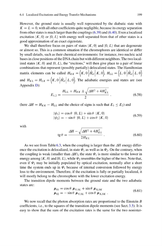
We shall therefore focus on pairs of states |K , 0 and |0, L that are degenerate
or almost so. This is a common situation if the chromophores are identical or differ
by small details, such as their chemical environments: for instance, two nucleic acid
bases in close positions of the DNA chain but with different neighbors. The two localized states |K , 0 and |0, L, the “excitons,” will then give place to a pair of linear
combinations that represent (possibly partially) delocalized states. The Hamiltonian
matrix elements can be called H K K =
K , 0
ˆ
H el
K , 0
, H L L =
L , 0
ˆ
H el
L , 0
and H K L = H L K =
K , 0
ˆ
H el
L , 0
. The adiabatic energies and states are (see
Appendix D):
E 1,2 =
H L L + H K K ±
ΔH 2 + 4H
2
K L
2
.
(6.58)
(here ΔH = H K K − H L L and the choice of signs is such that E 1 ≤ E 2 ) and
|ψ 1 = cos θ |0, L + sin θ |K , 0
|ψ 2 = − sin θ |0, L + cos θ |K , 0
(6.59)
with
tg θ =
ΔH −
ΔH 2 + 4H
2
K L
2H K L
.
(6.60)
As we see from Table 6.3, when the coupling is larger than the ΔH energy difference the excitation is delocalized, in state Ψ 1 as well as in Ψ 2 . On the contrary, when
the coupling is weak (smaller than ΔH ), the state Ψ 1 is more similar to the lower in
energy among |K , 0 and |0, L, while Ψ 2 resembles the higher of the two. Note that,
even if Ψ 2 may be initially populated by optical excitation, normally after a short
time the system ends up in Ψ 1 because of internal conversion followed by energy
loss to the environment. Therefore, if the excitation is fully or partially localized, it
will mostly belong to the chromophore with the lower excitation energy.
The transition dipole moments between the ground state and the two adiabatic
states are:
µ 01 = cos θ µ Y,0L + sin θ µ X,0K
µ 02 = − sin θ µ Y,0L + cos θ µ X,0K .
(6.61)
We now recall that the photon absorption rates are proportional to the Einstein B
coefficients, i.e., to the squares of the transition dipole moments (see Sect. 3.5). It is
easy to show that the sum of the excitation rates is the same for the two noninter-
199
However, the ground state is usually well represented by the diabatic state with
K = L = 0, with all other coefficients quite negligible, because its energy separation
from other states is much larger than the couplings (6.39) and (6.40). Even a localized
excitation |K , 0 or |0, L with energy well separated from that of other states is a
good approximation of an exact eigenstate.
We shall therefore focus on pairs of states |K , 0 and |0, L that are degenerate
or almost so. This is a common situation if the chromophores are identical or differ
by small details, such as their chemical environments: for instance, two nucleic acid
bases in close positions of the DNA chain but with different neighbors. The two localized states |K , 0 and |0, L, the “excitons,” will then give place to a pair of linear
combinations that represent (possibly partially) delocalized states. The Hamiltonian
matrix elements can be called H K K =
K , 0
ˆ
H el
K , 0
, H L L =
L , 0
ˆ
H el
L , 0
and H K L = H L K =
K , 0
ˆ
H el
L , 0
. The adiabatic energies and states are (see
Appendix D):
E 1,2 =
H L L + H K K ±
ΔH 2 + 4H
2
K L
2
.
(6.58)
(here ΔH = H K K − H L L and the choice of signs is such that E 1 ≤ E 2 ) and
|ψ 1 = cos θ |0, L + sin θ |K , 0
|ψ 2 = − sin θ |0, L + cos θ |K , 0
(6.59)
with
tg θ =
ΔH −
ΔH 2 + 4H
2
K L
2H K L
.
(6.60)
As we see from Table 6.3, when the coupling is larger than the ΔH energy difference the excitation is delocalized, in state Ψ 1 as well as in Ψ 2 . On the contrary, when
the coupling is weak (smaller than ΔH ), the state Ψ 1 is more similar to the lower in
energy among |K , 0 and |0, L, while Ψ 2 resembles the higher of the two. Note that,
even if Ψ 2 may be initially populated by optical excitation, normally after a short
time the system ends up in Ψ 1 because of internal conversion followed by energy
loss to the environment. Therefore, if the excitation is fully or partially localized, it
will mostly belong to the chromophore with the lower excitation energy.
The transition dipole moments between the ground state and the two adiabatic
states are:
µ 01 = cos θ µ Y,0L + sin θ µ X,0K
µ 02 = − sin θ µ Y,0L + cos θ µ X,0K .
(6.61)
We now recall that the photon absorption rates are proportional to the Einstein B
coefficients, i.e., to the squares of the transition dipole moments (see Sect. 3.5). It is
easy to show that the sum of the excitation rates is the same for the two noninter-