

190
6 Charge and Energy Transfer Processes
6.4.1 Group Functions
In this section we shall tackle the problem of defining localized excitations by introducing the concept of “group functions” with “strong orthogonality” conditions (see
McWeeny [11], Sect. 14.1). The advantage is that the matrix elements of the Hamiltonian are given by simple formulas and can be related to properties of the X and
Y subsystems, so leading to a better understanding of the energy transfer processes.
The group functions are antisymmetric electronic wavefunctions Ψ X,K and Ψ Y,L for
the X and Y subsystems, respectively. The space and spin coordinates of the n X electrons of X will be called x i and those of the n Y electrons of Y, y j . We build Ψ X,K and
Ψ Y,L as CI expansions using a set of orthogonal MOs, each of them being localized
on either the subsystem X or Y. Such MOs can be obtained for instance by HF or
CASSCF calculations for the whole system, followed by a localization procedure
based on rotations within each subset of doubly occupied, active or virtual orbitals.
Because of the limitations imposed by the preservation of orthogonality, a complete
localization will not be achieved unless X and Y are very far apart, but we assume
it is possible to attribute each MO to either X or Y (see Appendix E). We define the
subspaces S X and S Y , each spanned by all the Slater determinants of n S electrons
that only occupy MOs belonging to subsystem S. The Ψ X,J wavefunctions are built
with determinants of only one of the two subspaces and therefore belong to either
S X or S Y . Charge transfer configurations, with the numbers of electrons in X and Y
different from n X and n Y , are therefore not included in our treatment. We require
orthonormalization within each set of group functions:
Ψ X,K
Ψ X,K
= δ K ,K ,
Ψ Y,L
Ψ Y,L
= δ L ,L .
(6.28)
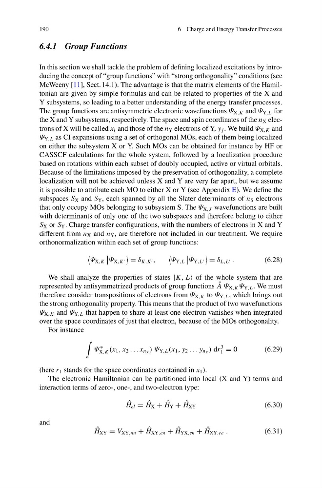
We shall analyze the properties of states |K , L of the whole system that are
represented by antisymmetrized products of group functions ˆ
A Ψ X,K Ψ Y,L . We must
therefore consider transpositions of electrons from Ψ X,K to Ψ Y,L , which brings out
the strong orthogonality property. This means that the product of two wavefunctions
Ψ X,K and Ψ Y,L that happen to share at least one electron vanishes when integrated
over the space coordinates of just that electron, because of the MOs orthogonality.
For instance
Ψ
∗
X,K (x 1 , x 2 . . . x n X ) Ψ Y,L (x 1 , y 2 . . . y n Y ) dr
3
1 = 0
(6.29)
(here r 1 stands for the space coordinates contained in x 1 ).
The electronic Hamiltonian can be partitioned into local (X and Y) terms and
interaction terms of zero-, one-, and two-electron type:
ˆ
H el = ˆ
H X + ˆ
H Y + ˆ
H XY
(6.30)
and
ˆ
H XY = V XY,nn + ˆ
H XY,en + ˆ
H YX,en + ˆ
H XY,ee .
(6.31)
6 Charge and Energy Transfer Processes
6.4.1 Group Functions
In this section we shall tackle the problem of defining localized excitations by introducing the concept of “group functions” with “strong orthogonality” conditions (see
McWeeny [11], Sect. 14.1). The advantage is that the matrix elements of the Hamiltonian are given by simple formulas and can be related to properties of the X and
Y subsystems, so leading to a better understanding of the energy transfer processes.
The group functions are antisymmetric electronic wavefunctions Ψ X,K and Ψ Y,L for
the X and Y subsystems, respectively. The space and spin coordinates of the n X electrons of X will be called x i and those of the n Y electrons of Y, y j . We build Ψ X,K and
Ψ Y,L as CI expansions using a set of orthogonal MOs, each of them being localized
on either the subsystem X or Y. Such MOs can be obtained for instance by HF or
CASSCF calculations for the whole system, followed by a localization procedure
based on rotations within each subset of doubly occupied, active or virtual orbitals.
Because of the limitations imposed by the preservation of orthogonality, a complete
localization will not be achieved unless X and Y are very far apart, but we assume
it is possible to attribute each MO to either X or Y (see Appendix E). We define the
subspaces S X and S Y , each spanned by all the Slater determinants of n S electrons
that only occupy MOs belonging to subsystem S. The Ψ X,J wavefunctions are built
with determinants of only one of the two subspaces and therefore belong to either
S X or S Y . Charge transfer configurations, with the numbers of electrons in X and Y
different from n X and n Y , are therefore not included in our treatment. We require
orthonormalization within each set of group functions:
Ψ X,K
Ψ X,K
= δ K ,K ,
Ψ Y,L
Ψ Y,L
= δ L ,L .
(6.28)
We shall analyze the properties of states |K , L of the whole system that are
represented by antisymmetrized products of group functions ˆ
A Ψ X,K Ψ Y,L . We must
therefore consider transpositions of electrons from Ψ X,K to Ψ Y,L , which brings out
the strong orthogonality property. This means that the product of two wavefunctions
Ψ X,K and Ψ Y,L that happen to share at least one electron vanishes when integrated
over the space coordinates of just that electron, because of the MOs orthogonality.
For instance
Ψ
∗
X,K (x 1 , x 2 . . . x n X ) Ψ Y,L (x 1 , y 2 . . . y n Y ) dr
3
1 = 0
(6.29)
(here r 1 stands for the space coordinates contained in x 1 ).
The electronic Hamiltonian can be partitioned into local (X and Y) terms and
interaction terms of zero-, one-, and two-electron type:
ˆ
H el = ˆ
H X + ˆ
H Y + ˆ
H XY
(6.30)
and
ˆ
H XY = V XY,nn + ˆ
H XY,en + ˆ
H YX,en + ˆ
H XY,ee .
(6.31)