

5.4 Conical Intersections
167
result for Ω
(C)
k
does not contradict what is reported in Sect. 5.4.3. In fact, the Stokes
theorem requires the function ˜
g kk to be differentiable on S C , so Eq.(5.79) is only
applicable if the surface S C does not contain the intersection point, where ˜
g kk has a
singularity.
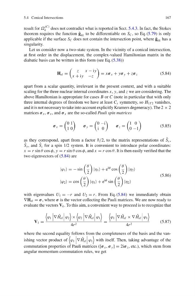
Let us consider now a two-state system. In the vicinity of a conical intersection,
at first order in the displacement, the complex-valued Hamiltonian matrix in the
diabatic basis can be written in this form (see Eq. (5.38))
H el =
z x − iy
x + iy −z
= xσ x + yσ y + zσ z
(5.84)
apart from a scalar quantity, irrelevant in the present context, and with a suitable
scaling for the three nuclear internal coordinates x, y, and z we are considering. The
above Hamiltonian is appropriate for cases B or C (note in particular that with only
three internal degrees of freedom we have at least C s symmetry, so H 1T 2 vanishes,
and it is not necessary to take into account explicitly Kramers degeneracy). The 2 × 2
matrices σ x , σ x , and σ x are the so-called Pauli spin matrices
σ x =
0 1
1 0
σ y =
0 −i
i 0
σ z =
1 0
0 −1
(5.85)
as they correspond, apart from a factor /2, to the matrix representations of ˆ
S x ,
ˆ
S y , and ˆ
S z for a spin 1/2 system. It is convenient to introduce polar coordinates:
x = r sin θ cos φ, y = r sin θ cos φ, and x = r cos θ . It is then easily verified that the
two eigenvectors of (5.84) are
|ϕ 1 = − sin
θ
2
|η 1 + e
iφ cos
θ
2
|η 2
|ϕ 2 = cos
θ
2
|η 1 + e
iφ sin
θ
2
|η 2
(5.86)
with eigenvalues U 1 = −r and U 2 = r . From Eq.(5.84) we immediately obtain
∇H el = σ , where σ is the vector collecting the Pauli matrices. We are now ready to
evaluate the vectors V k . To this aim, a convenient way to proceed is to recognize that
V 1 =
ϕ 1
∇ ˆ
H el
ϕ 2
×
ϕ 2
∇ ˆ
H el
ϕ 1
4r 2
=
ϕ 1
∇ ˆ
H el × ∇ ˆ
H el
ϕ 1
4r 2
(5.87)
where the second equality follows from the completeness of the basis and the vanishing vector product of
ϕ 1
∇ ˆ
H el
ϕ 1
with itself. Then, taking advantage of the
commutation properties of Pauli matrices ([σ x , σ y ] = 2iσ z , etc.), which stem from
angular momentum commutation rules, we get
167
result for Ω
(C)
k
does not contradict what is reported in Sect. 5.4.3. In fact, the Stokes
theorem requires the function ˜
g kk to be differentiable on S C , so Eq.(5.79) is only
applicable if the surface S C does not contain the intersection point, where ˜
g kk has a
singularity.
Let us consider now a two-state system. In the vicinity of a conical intersection,
at first order in the displacement, the complex-valued Hamiltonian matrix in the
diabatic basis can be written in this form (see Eq. (5.38))
H el =
z x − iy
x + iy −z
= xσ x + yσ y + zσ z
(5.84)
apart from a scalar quantity, irrelevant in the present context, and with a suitable
scaling for the three nuclear internal coordinates x, y, and z we are considering. The
above Hamiltonian is appropriate for cases B or C (note in particular that with only
three internal degrees of freedom we have at least C s symmetry, so H 1T 2 vanishes,
and it is not necessary to take into account explicitly Kramers degeneracy). The 2 × 2
matrices σ x , σ x , and σ x are the so-called Pauli spin matrices
σ x =
0 1
1 0
σ y =
0 −i
i 0
σ z =
1 0
0 −1
(5.85)
as they correspond, apart from a factor /2, to the matrix representations of ˆ
S x ,
ˆ
S y , and ˆ
S z for a spin 1/2 system. It is convenient to introduce polar coordinates:
x = r sin θ cos φ, y = r sin θ cos φ, and x = r cos θ . It is then easily verified that the
two eigenvectors of (5.84) are
|ϕ 1 = − sin
θ
2
|η 1 + e
iφ cos
θ
2
|η 2
|ϕ 2 = cos
θ
2
|η 1 + e
iφ sin
θ
2
|η 2
(5.86)
with eigenvalues U 1 = −r and U 2 = r . From Eq.(5.84) we immediately obtain
∇H el = σ , where σ is the vector collecting the Pauli matrices. We are now ready to
evaluate the vectors V k . To this aim, a convenient way to proceed is to recognize that
V 1 =
ϕ 1
∇ ˆ
H el
ϕ 2
×
ϕ 2
∇ ˆ
H el
ϕ 1
4r 2
=
ϕ 1
∇ ˆ
H el × ∇ ˆ
H el
ϕ 1
4r 2
(5.87)
where the second equality follows from the completeness of the basis and the vanishing vector product of
ϕ 1
∇ ˆ
H el
ϕ 1
with itself. Then, taking advantage of the
commutation properties of Pauli matrices ([σ x , σ y ] = 2iσ z , etc.), which stem from
angular momentum commutation rules, we get