

5.4 Conical Intersections
161
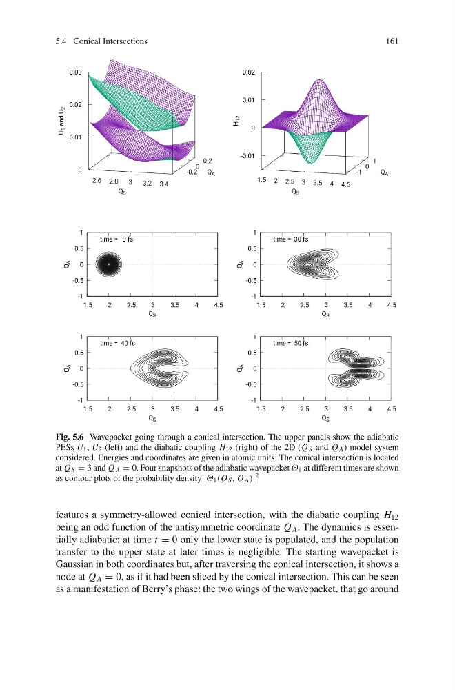
Fig. 5.6 Wavepacket going through a conical intersection. The upper panels show the adiabatic
PESs U 1 , U 2 (left) and the diabatic coupling H 12 (right) of the 2D (Q S and Q A ) model system
considered. Energies and coordinates are given in atomic units. The conical intersection is located
at Q S = 3 and Q A = 0. Four snapshots of the adiabatic wavepacket Θ 1 at different times are shown
as contour plots of the probability density |Θ 1 (Q S , Q A )|
2
features a symmetry-allowed conical intersection, with the diabatic coupling H 12
being an odd function of the antisymmetric coordinate Q A . The dynamics is essentially adiabatic: at time t = 0 only the lower state is populated, and the population
transfer to the upper state at later times is negligible. The starting wavepacket is
Gaussian in both coordinates but, after traversing the conical intersection, it shows a
node at Q A = 0, as if it had been sliced by the conical intersection. This can be seen
as a manifestation of Berry’s phase: the two wings of the wavepacket, that go around
161
Fig. 5.6 Wavepacket going through a conical intersection. The upper panels show the adiabatic
PESs U 1 , U 2 (left) and the diabatic coupling H 12 (right) of the 2D (Q S and Q A ) model system
considered. Energies and coordinates are given in atomic units. The conical intersection is located
at Q S = 3 and Q A = 0. Four snapshots of the adiabatic wavepacket Θ 1 at different times are shown
as contour plots of the probability density |Θ 1 (Q S , Q A )|
2
features a symmetry-allowed conical intersection, with the diabatic coupling H 12
being an odd function of the antisymmetric coordinate Q A . The dynamics is essentially adiabatic: at time t = 0 only the lower state is populated, and the population
transfer to the upper state at later times is negligible. The starting wavepacket is
Gaussian in both coordinates but, after traversing the conical intersection, it shows a
node at Q A = 0, as if it had been sliced by the conical intersection. This can be seen
as a manifestation of Berry’s phase: the two wings of the wavepacket, that go around