

5.4 Conical Intersections
159
y
x
γ
y
x
γ
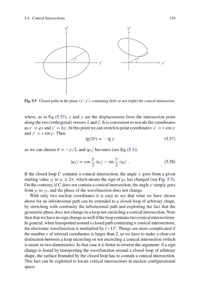
Fig. 5.5 Closed paths in the plane (x , y ), containing (left) or not (right) the conical intersection
where, as in Eq. (5.37), x and y are the displacements from the intersection point
along the two (orthogonal) versors ˆ
x and ˆ
y. It is convenient to rescale the coordinates
as x
= qx and y
= hy. At this point we can switch to polar coordinates: x
= r cos γ
and y
= r sin γ . Then
tg(2θ) = − tg γ
(5.57)
so we can choose θ = −γ /2, and |ϕ 1 becomes (see Eq. (5.1))
|ϕ 1 = cos
γ
2
|η 1 − sin
γ
2
|η 2 .
(5.58)
If the closed loop C contains a conical intersection, the angle γ goes from a given
starting value γ i to γ i ± 2π , which means the sign of ϕ 1 has changed (see Fig. 5.5).
On the contrary, if C does not contain a conical intersection, the angle γ simply goes
from γ i to γ i , and the phase of the wavefunction does not change.
With only two nuclear coordinates it is easy to see that what we have shown
above for an infinitesimal path can be extended to a closed loop of arbitrary shape,
by stretching with continuity the infinitesimal path and exploiting the fact that the
geometric phase does not change in a loop not encircling a conical intersection. Note
then that we have no sign change as well if the loop contains two conical intersections.
In general, when transported around a closed path containing n conical intersections,
the electronic wavefunction is multiplied by (−1)
n . Things are more complicated if
the number s of internal coordinates is larger than 2, as we have to make a clear-cut
distinction between a loop encircling or not encircling a conical intersection (which
is easier in two dimensions). In that case it is better to reverse the argument: if a sign
change is found by transporting the wavefunction around a closed loop of arbitrary
shape, the surface bounded by the closed loop has to contain a conical intersection.
This fact can be exploited to locate conical intersections in nuclear configurational
space.
159
y
x
γ
y
x
γ
Fig. 5.5 Closed paths in the plane (x , y ), containing (left) or not (right) the conical intersection
where, as in Eq. (5.37), x and y are the displacements from the intersection point
along the two (orthogonal) versors ˆ
x and ˆ
y. It is convenient to rescale the coordinates
as x
= qx and y
= hy. At this point we can switch to polar coordinates: x
= r cos γ
and y
= r sin γ . Then
tg(2θ) = − tg γ
(5.57)
so we can choose θ = −γ /2, and |ϕ 1 becomes (see Eq. (5.1))
|ϕ 1 = cos
γ
2
|η 1 − sin
γ
2
|η 2 .
(5.58)
If the closed loop C contains a conical intersection, the angle γ goes from a given
starting value γ i to γ i ± 2π , which means the sign of ϕ 1 has changed (see Fig. 5.5).
On the contrary, if C does not contain a conical intersection, the angle γ simply goes
from γ i to γ i , and the phase of the wavefunction does not change.
With only two nuclear coordinates it is easy to see that what we have shown
above for an infinitesimal path can be extended to a closed loop of arbitrary shape,
by stretching with continuity the infinitesimal path and exploiting the fact that the
geometric phase does not change in a loop not encircling a conical intersection. Note
then that we have no sign change as well if the loop contains two conical intersections.
In general, when transported around a closed path containing n conical intersections,
the electronic wavefunction is multiplied by (−1)
n . Things are more complicated if
the number s of internal coordinates is larger than 2, as we have to make a clear-cut
distinction between a loop encircling or not encircling a conical intersection (which
is easier in two dimensions). In that case it is better to reverse the argument: if a sign
change is found by transporting the wavefunction around a closed loop of arbitrary
shape, the surface bounded by the closed loop has to contain a conical intersection.
This fact can be exploited to locate conical intersections in nuclear configurational
space.