

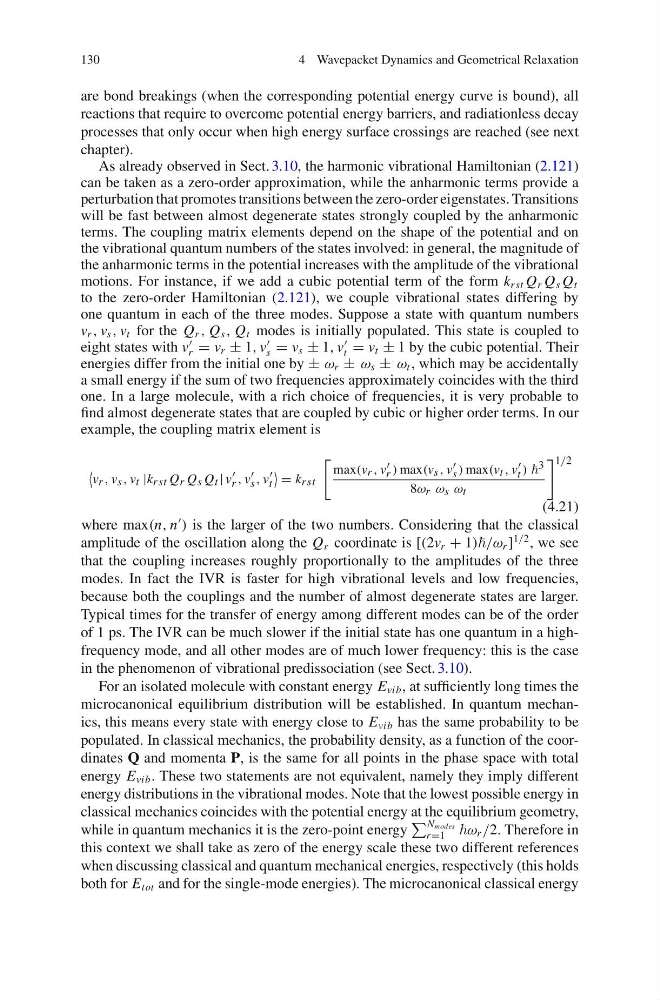
130
4 Wavepacket Dynamics and Geometrical Relaxation
are bond breakings (when the corresponding potential energy curve is bound), all
reactions that require to overcome potential energy barriers, and radiationless decay
processes that only occur when high energy surface crossings are reached (see next
chapter).
As already observed in Sect. 3.10, the harmonic vibrational Hamiltonian (2.121)
can be taken as a zero-order approximation, while the anharmonic terms provide a
perturbation that promotes transitions between the zero-order eigenstates. Transitions
will be fast between almost degenerate states strongly coupled by the anharmonic
terms. The coupling matrix elements depend on the shape of the potential and on
the vibrational quantum numbers of the states involved: in general, the magnitude of
the anharmonic terms in the potential increases with the amplitude of the vibrational
motions. For instance, if we add a cubic potential term of the form k rst Q r Q s Q t
to the zero-order Hamiltonian (2.121), we couple vibrational states differing by
one quantum in each of the three modes. Suppose a state with quantum numbers
v r , v s , v t for the Q r , Q s , Q t modes is initially populated. This state is coupled to
eight states with v
r = v r ± 1, v
s = v s ± 1, v
t = v t ± 1 by the cubic potential. Their
energies differ from the initial one by ± ω r ± ω s ± ω t , which may be accidentally
a small energy if the sum of two frequencies approximately coincides with the third
one. In a large molecule, with a rich choice of frequencies, it is very probable to
find almost degenerate states that are coupled by cubic or higher order terms. In our
example, the coupling matrix element is
v r , v s , v t |k rst Q r Q s Q t | v
r , v
s , v
t
= k rst
max(v r , v
r ) max(v s , v
s ) max(v t , v
t ) 3
8ω r ω s ω t
1/2
(4.21)
where max(n, n
) is the larger of the two numbers. Considering that the classical
amplitude of the oscillation along the Q r coordinate is [(2v r + 1)/ω r ]
1/2 , we see
that the coupling increases roughly proportionally to the amplitudes of the three
modes. In fact the IVR is faster for high vibrational levels and low frequencies,
because both the couplings and the number of almost degenerate states are larger.
Typical times for the transfer of energy among different modes can be of the order
of 1 ps. The IVR can be much slower if the initial state has one quantum in a highfrequency mode, and all other modes are of much lower frequency: this is the case
in the phenomenon of vibrational predissociation (see Sect. 3.10).
For an isolated molecule with constant energy E vib , at sufficiently long times the
microcanonical equilibrium distribution will be established. In quantum mechanics, this means every state with energy close to E vib has the same probability to be
populated. In classical mechanics, the probability density, as a function of the coordinates Q and momenta P, is the same for all points in the phase space with total
energy E vib . These two statements are not equivalent, namely they imply different
energy distributions in the vibrational modes. Note that the lowest possible energy in
classical mechanics coincides with the potential energy at the equilibrium geometry,
while in quantum mechanics it is the zero-point energy
N modes
r =1 ω r /2. Therefore in
this context we shall take as zero of the energy scale these two different references
when discussing classical and quantum mechanical energies, respectively (this holds
both for E tot and for the single-mode energies). The microcanonical classical energy
4 Wavepacket Dynamics and Geometrical Relaxation
are bond breakings (when the corresponding potential energy curve is bound), all
reactions that require to overcome potential energy barriers, and radiationless decay
processes that only occur when high energy surface crossings are reached (see next
chapter).
As already observed in Sect. 3.10, the harmonic vibrational Hamiltonian (2.121)
can be taken as a zero-order approximation, while the anharmonic terms provide a
perturbation that promotes transitions between the zero-order eigenstates. Transitions
will be fast between almost degenerate states strongly coupled by the anharmonic
terms. The coupling matrix elements depend on the shape of the potential and on
the vibrational quantum numbers of the states involved: in general, the magnitude of
the anharmonic terms in the potential increases with the amplitude of the vibrational
motions. For instance, if we add a cubic potential term of the form k rst Q r Q s Q t
to the zero-order Hamiltonian (2.121), we couple vibrational states differing by
one quantum in each of the three modes. Suppose a state with quantum numbers
v r , v s , v t for the Q r , Q s , Q t modes is initially populated. This state is coupled to
eight states with v
r = v r ± 1, v
s = v s ± 1, v
t = v t ± 1 by the cubic potential. Their
energies differ from the initial one by ± ω r ± ω s ± ω t , which may be accidentally
a small energy if the sum of two frequencies approximately coincides with the third
one. In a large molecule, with a rich choice of frequencies, it is very probable to
find almost degenerate states that are coupled by cubic or higher order terms. In our
example, the coupling matrix element is
v r , v s , v t |k rst Q r Q s Q t | v
r , v
s , v
t
= k rst
max(v r , v
r ) max(v s , v
s ) max(v t , v
t ) 3
8ω r ω s ω t
1/2
(4.21)
where max(n, n
) is the larger of the two numbers. Considering that the classical
amplitude of the oscillation along the Q r coordinate is [(2v r + 1)/ω r ]
1/2 , we see
that the coupling increases roughly proportionally to the amplitudes of the three
modes. In fact the IVR is faster for high vibrational levels and low frequencies,
because both the couplings and the number of almost degenerate states are larger.
Typical times for the transfer of energy among different modes can be of the order
of 1 ps. The IVR can be much slower if the initial state has one quantum in a highfrequency mode, and all other modes are of much lower frequency: this is the case
in the phenomenon of vibrational predissociation (see Sect. 3.10).
For an isolated molecule with constant energy E vib , at sufficiently long times the
microcanonical equilibrium distribution will be established. In quantum mechanics, this means every state with energy close to E vib has the same probability to be
populated. In classical mechanics, the probability density, as a function of the coordinates Q and momenta P, is the same for all points in the phase space with total
energy E vib . These two statements are not equivalent, namely they imply different
energy distributions in the vibrational modes. Note that the lowest possible energy in
classical mechanics coincides with the potential energy at the equilibrium geometry,
while in quantum mechanics it is the zero-point energy
N modes
r =1 ω r /2. Therefore in
this context we shall take as zero of the energy scale these two different references
when discussing classical and quantum mechanical energies, respectively (this holds
both for E tot and for the single-mode energies). The microcanonical classical energy