

126
4 Wavepacket Dynamics and Geometrical Relaxation
components of a wavefunction (here, the vibrational eigenstates) do not keep the
same relationships among them while evolving in time. In the case of anharmonic
potentials the reason is dephasing (i.e., change of the relative phases) of the coefficients of the eigenstates: in fact, the coefficients do not change with a common time
period as those of Eq. (4.12), because the vibrational levels in the Morse potential
are not equispaced. This is confirmed by comparing the dynamics triggered by the
τ = 10 and τ = 60 fs pulses: with the latter, as already seen in the harmonic case,
very few vibrational eigenstates are significantly populated (those with v = 39, 40
and 41), so the wavepacket is delocalized and the amplitude of the R oscillations
is initially smaller than with the 10 fs pulse. However, the amplitude decreases much
more slowly than with the 10 fs pulse and the animation shows almost no decoherence effects. The reason is that dephasing is minimal, because the E 40 − E 39 and
E 41 − E 40 energy differences are almost equal. Decoherence is much faster when
the wavepacket is expanded on a dozen of states, as with the shorter pulse, because
then the spread in the energy differences is larger.
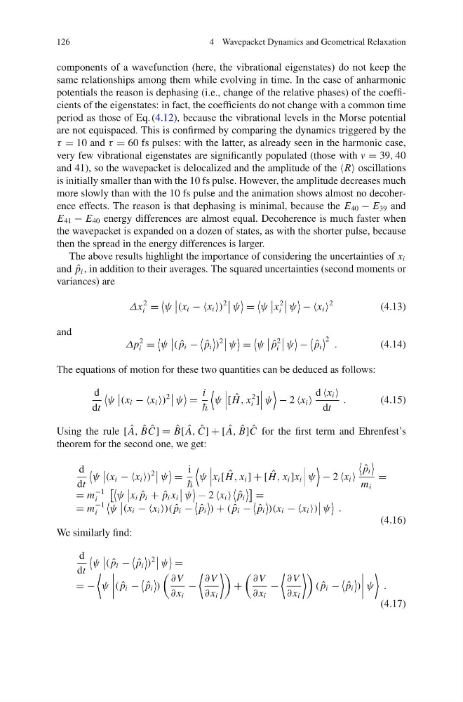
The above results highlight the importance of considering the uncertainties of x i
and ˆ
p i , in addition to their averages. The squared uncertainties (second moments or
variances) are
Δx
2
i =
ψ
(x i − x i )
2
ψ
=
ψ
x
2
i
ψ
− x i
2
(4.13)
and
Δp
2
i =
ψ
( ˆ
p i −
ˆ
p i
)
2
ψ
=
ψ
ˆ
p
2
i
ψ
−
ˆ
p i
2 .
(4.14)
The equations of motion for these two quantities can be deduced as follows:
d
dt
ψ
(x i − x i )
2
ψ
=
i
ψ
[ ˆ
H , x
2
i ]
ψ
− 2 x i
d x i
dt
.
(4.15)
Using the rule [ ˆ
A, ˆ
B ˆ
C] = ˆ
B[ ˆ
A, ˆ
C] + [ ˆ
A, ˆ
B] ˆ
C for the first term and Ehrenfest’s
theorem for the second one, we get:
d
dt
ψ
(x i − x i )
2
ψ
=
i
ψ
x i [ ˆ
H , x i ] + [ ˆ
H , x i ]x i
ψ
− 2 x i
ˆ
p i
m i
=
= m
−1
i
ψ
x i ˆ
p i + ˆ
p i x i
ψ
− 2 x i
ˆ
p i
=
= m
−1
i
ψ
(x i − x i )( ˆ
p i −
ˆ
p i
) + ( ˆ
p i −
ˆ
p i
)(x i − x i )
ψ
.
(4.16)
We similarly find:
d
dt
ψ
( ˆ
p i −
ˆ
p i
)
2
ψ
=
= −
ψ
( ˆ
p i −
ˆ
p i
)
∂ V
∂ x i
−
∂ V
∂ x i
+
∂ V
∂ x i
−
∂ V
∂ x i
( ˆ
p i −
ˆ
p i
)
ψ
.
(4.17)
4 Wavepacket Dynamics and Geometrical Relaxation
components of a wavefunction (here, the vibrational eigenstates) do not keep the
same relationships among them while evolving in time. In the case of anharmonic
potentials the reason is dephasing (i.e., change of the relative phases) of the coefficients of the eigenstates: in fact, the coefficients do not change with a common time
period as those of Eq. (4.12), because the vibrational levels in the Morse potential
are not equispaced. This is confirmed by comparing the dynamics triggered by the
τ = 10 and τ = 60 fs pulses: with the latter, as already seen in the harmonic case,
very few vibrational eigenstates are significantly populated (those with v = 39, 40
and 41), so the wavepacket is delocalized and the amplitude of the R oscillations
is initially smaller than with the 10 fs pulse. However, the amplitude decreases much
more slowly than with the 10 fs pulse and the animation shows almost no decoherence effects. The reason is that dephasing is minimal, because the E 40 − E 39 and
E 41 − E 40 energy differences are almost equal. Decoherence is much faster when
the wavepacket is expanded on a dozen of states, as with the shorter pulse, because
then the spread in the energy differences is larger.
The above results highlight the importance of considering the uncertainties of x i
and ˆ
p i , in addition to their averages. The squared uncertainties (second moments or
variances) are
Δx
2
i =
ψ
(x i − x i )
2
ψ
=
ψ
x
2
i
ψ
− x i
2
(4.13)
and
Δp
2
i =
ψ
( ˆ
p i −
ˆ
p i
)
2
ψ
=
ψ
ˆ
p
2
i
ψ
−
ˆ
p i
2 .
(4.14)
The equations of motion for these two quantities can be deduced as follows:
d
dt
ψ
(x i − x i )
2
ψ
=
i
ψ
[ ˆ
H , x
2
i ]
ψ
− 2 x i
d x i
dt
.
(4.15)
Using the rule [ ˆ
A, ˆ
B ˆ
C] = ˆ
B[ ˆ
A, ˆ
C] + [ ˆ
A, ˆ
B] ˆ
C for the first term and Ehrenfest’s
theorem for the second one, we get:
d
dt
ψ
(x i − x i )
2
ψ
=
i
ψ
x i [ ˆ
H , x i ] + [ ˆ
H , x i ]x i
ψ
− 2 x i
ˆ
p i
m i
=
= m
−1
i
ψ
x i ˆ
p i + ˆ
p i x i
ψ
− 2 x i
ˆ
p i
=
= m
−1
i
ψ
(x i − x i )( ˆ
p i −
ˆ
p i
) + ( ˆ
p i −
ˆ
p i
)(x i − x i )
ψ
.
(4.16)
We similarly find:
d
dt
ψ
( ˆ
p i −
ˆ
p i
)
2
ψ
=
= −
ψ
( ˆ
p i −
ˆ
p i
)
∂ V
∂ x i
−
∂ V
∂ x i
+
∂ V
∂ x i
−
∂ V
∂ x i
( ˆ
p i −
ˆ
p i
)
ψ
.
(4.17)