

110
3 Electronic Excitation and Decay
exponential fit
numerical simulation
time, fs
5000
4000
3000
2000
0
1000
1
0.8
0.6
0.4
0.2
0
exponential fit
numerical simulation
time, fs
P
B
(t)
5000
4000
3000
2000
0
1000
1
0.8
0.6
0.4
0.2
0
P
B
(t)
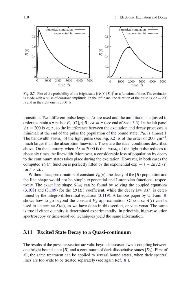
Fig. 3.7 Plot of the probability of the bright state ||Ψ (t) |B |
2 as a function of time. The excitation
is made with a pulse of constant amplitude. In the left panel the duration of the pulse is Δt = 200
fs and in the right one is 2000 fs
transition. Two different pulse lengths Δt are used and the amplitude is adjusted in
order to obtain a π pulse: E 0 G |μ| B Δt = π (see end of Sect. 3.3). In the left panel
Δt = 200 fs τ , so the interference between the excitation and decay processes is
minimal: at the end of the pulse the population of the bound state, P B , is almost 1.
The bandwidth FWHM ω of the light pulse (see Fig. 3.2) is of the order of 200 cm
−1 ,
much larger than the absorption linewidth. These are the ideal conditions described
above. On the contrary, when Δt = 2000 fs the FWHM ω of the light pulse reduces to
about six times the linewidth. Moreover, a considerable loss of population by decay
to the continuum states takes place during the excitation. However, in both cases the
computed P B (t) function is perfectly fitted by the exponential exp[−(t − Δt/2)/τ ]
for t > Δt.
Without the approximation of constant V B (ε), the decay of the |B population and
the line shape would not be simple exponential and Lorentzian functions, respectively. The exact line shape S(ω) can be found by solving the coupled equations
(3.108) and (3.109) for the B |E coefficient, while the decay law A(t) is determined by the integro-differential equation (3.119). A famous paper by U. Fano [8]
shows how to go beyond the constant V B approximation. Of course A(t) can be
used to determine S(ω), as we have done in this section, or vice versa. The same
is true if either quantity is determined experimentally: in principle, high-resolution
spectroscopy or time-resolved techniques yield the same information.
3.11 Excited State Decay to a Quasi-continuum
The results of the previous section are valid beyond the case of weak coupling between
one bright bound state |B and a continuum of dark dissociative states |D ε . First of
all, the same treatment can be applied to several bound states, when their spectral
lines are too wide to be treated separately (see again Ref. [8]).
3 Electronic Excitation and Decay
exponential fit
numerical simulation
time, fs
5000
4000
3000
2000
0
1000
1
0.8
0.6
0.4
0.2
0
exponential fit
numerical simulation
time, fs
P
B
(t)
5000
4000
3000
2000
0
1000
1
0.8
0.6
0.4
0.2
0
P
B
(t)
Fig. 3.7 Plot of the probability of the bright state ||Ψ (t) |B |
2 as a function of time. The excitation
is made with a pulse of constant amplitude. In the left panel the duration of the pulse is Δt = 200
fs and in the right one is 2000 fs
transition. Two different pulse lengths Δt are used and the amplitude is adjusted in
order to obtain a π pulse: E 0 G |μ| B Δt = π (see end of Sect. 3.3). In the left panel
Δt = 200 fs τ , so the interference between the excitation and decay processes is
minimal: at the end of the pulse the population of the bound state, P B , is almost 1.
The bandwidth FWHM ω of the light pulse (see Fig. 3.2) is of the order of 200 cm
−1 ,
much larger than the absorption linewidth. These are the ideal conditions described
above. On the contrary, when Δt = 2000 fs the FWHM ω of the light pulse reduces to
about six times the linewidth. Moreover, a considerable loss of population by decay
to the continuum states takes place during the excitation. However, in both cases the
computed P B (t) function is perfectly fitted by the exponential exp[−(t − Δt/2)/τ ]
for t > Δt.
Without the approximation of constant V B (ε), the decay of the |B population and
the line shape would not be simple exponential and Lorentzian functions, respectively. The exact line shape S(ω) can be found by solving the coupled equations
(3.108) and (3.109) for the B |E coefficient, while the decay law A(t) is determined by the integro-differential equation (3.119). A famous paper by U. Fano [8]
shows how to go beyond the constant V B approximation. Of course A(t) can be
used to determine S(ω), as we have done in this section, or vice versa. The same
is true if either quantity is determined experimentally: in principle, high-resolution
spectroscopy or time-resolved techniques yield the same information.
3.11 Excited State Decay to a Quasi-continuum
The results of the previous section are valid beyond the case of weak coupling between
one bright bound state |B and a continuum of dark dissociative states |D ε . First of
all, the same treatment can be applied to several bound states, when their spectral
lines are too wide to be treated separately (see again Ref. [8]).