

100
3 Electronic Excitation and Decay
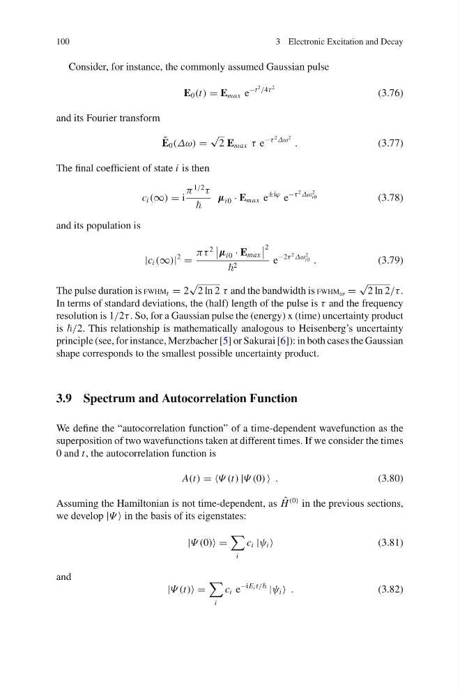
Consider, for instance, the commonly assumed Gaussian pulse
E 0 (t) = E max e
−t
2 /4τ
2
(3.76)
and its Fourier transform
˜
E 0 (Δω) =
√
2 E max τ e
−τ
2 Δω
2 .
(3.77)
The final coefficient of state i is then
c i (∞) = i
π
1/2
τ
µ i0 · E max e
±iϕ e
−τ
2 Δω
2
i0
(3.78)
and its population is
|c i (∞)|
2
=
πτ
2
µ i0 · E max
2
2
e
−2τ
2 Δω
2
i0 .
(3.79)
The pulse duration is FWHM t = 2
√
2 ln 2 τ and the bandwidth is FWHM ω =
√
2 ln 2/τ .
In terms of standard deviations, the (half) length of the pulse is τ and the frequency
resolution is 1/2τ . So, for a Gaussian pulse the (energy) x (time) uncertainty product
is /2. This relationship is mathematically analogous to Heisenberg’s uncertainty
principle (see, for instance, Merzbacher [5] or Sakurai [6]): in both cases the Gaussian
shape corresponds to the smallest possible uncertainty product.
3.9 Spectrum and Autocorrelation Function
We define the “autocorrelation function” of a time-dependent wavefunction as the
superposition of two wavefunctions taken at different times. If we consider the times
0 and t, the autocorrelation function is
A(t) = Ψ (t) |Ψ (0) .
(3.80)
Assuming the Hamiltonian is not time-dependent, as ˆ
H
(0) in the previous sections,
we develop |Ψ in the basis of its eigenstates:
|Ψ (0) =
i
c i |ψ i
(3.81)
and
|Ψ (t) =
i
c i e
−iE i t/
|ψ i .
(3.82)
3 Electronic Excitation and Decay
Consider, for instance, the commonly assumed Gaussian pulse
E 0 (t) = E max e
−t
2 /4τ
2
(3.76)
and its Fourier transform
˜
E 0 (Δω) =
√
2 E max τ e
−τ
2 Δω
2 .
(3.77)
The final coefficient of state i is then
c i (∞) = i
π
1/2
τ
µ i0 · E max e
±iϕ e
−τ
2 Δω
2
i0
(3.78)
and its population is
|c i (∞)|
2
=
πτ
2
µ i0 · E max
2
2
e
−2τ
2 Δω
2
i0 .
(3.79)
The pulse duration is FWHM t = 2
√
2 ln 2 τ and the bandwidth is FWHM ω =
√
2 ln 2/τ .
In terms of standard deviations, the (half) length of the pulse is τ and the frequency
resolution is 1/2τ . So, for a Gaussian pulse the (energy) x (time) uncertainty product
is /2. This relationship is mathematically analogous to Heisenberg’s uncertainty
principle (see, for instance, Merzbacher [5] or Sakurai [6]): in both cases the Gaussian
shape corresponds to the smallest possible uncertainty product.
3.9 Spectrum and Autocorrelation Function
We define the “autocorrelation function” of a time-dependent wavefunction as the
superposition of two wavefunctions taken at different times. If we consider the times
0 and t, the autocorrelation function is
A(t) = Ψ (t) |Ψ (0) .
(3.80)
Assuming the Hamiltonian is not time-dependent, as ˆ
H
(0) in the previous sections,
we develop |Ψ in the basis of its eigenstates:
|Ψ (0) =
i
c i |ψ i
(3.81)
and
|Ψ (t) =
i
c i e
−iE i t/
|ψ i .
(3.82)