

2.4 Numerical Integration of the Schrödinger Equation
75
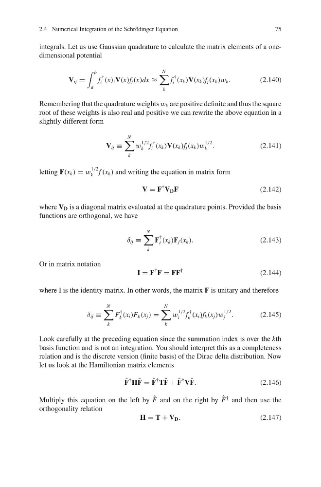
integrals. Let us use Gaussian quadrature to calculate the matrix elements of a onedimensional potential
V ij =
b
a
f
†
i (x) i V(x)f j (x)dx ≈
N
k
f
†
i (x k )V(x k )f j (x k )w k .
(2.140)
Remembering that the quadrature weights w k are positive definite and thus the square
root of these weights is also real and positive we can rewrite the above equation in a
slightly different form
V ij ≡
N
k
w
1/2
k f
†
i (x k )V(x k )f j (x k )w
1/2
k .
(2.141)
letting F(x k ) = w
1/2
k f (x k ) and writing the equation in matrix form
V = F
† V D F
(2.142)
where V D is a diagonal matrix evaluated at the quadrature points. Provided the basis
functions are orthogonal, we have
δ ij ≡
N
k
F
†
i (x k )F j (x k ).
(2.143)
Or in matrix notation
I = F
† F = FF
†
(2.144)
where I is the identity matrix. In other words, the matrix F is unitary and therefore
δ ij ≡
N
k
F
†
k (x i )F k (x j ) =
N
k
w
1/2
i f
†
k (x i )f k (x j )w
1/2
j .
(2.145)
Look carefully at the preceding equation since the summation index is over the kth
basis function and is not an integration. You should interpret this as a completeness
relation and is the discrete version (finite basis) of the Dirac delta distribution. Now
let us look at the Hamiltonian matrix elements
ˆ
F
† H ˆ
F = ˆ
F
† T ˆ
F + ˆ
F
† V ˆ
F.
(2.146)
Multiply this equation on the left by ˆ
F and on the right by ˆ
F
† and then use the
orthogonality relation
H = T + V D .
(2.147)
75
integrals. Let us use Gaussian quadrature to calculate the matrix elements of a onedimensional potential
V ij =
b
a
f
†
i (x) i V(x)f j (x)dx ≈
N
k
f
†
i (x k )V(x k )f j (x k )w k .
(2.140)
Remembering that the quadrature weights w k are positive definite and thus the square
root of these weights is also real and positive we can rewrite the above equation in a
slightly different form
V ij ≡
N
k
w
1/2
k f
†
i (x k )V(x k )f j (x k )w
1/2
k .
(2.141)
letting F(x k ) = w
1/2
k f (x k ) and writing the equation in matrix form
V = F
† V D F
(2.142)
where V D is a diagonal matrix evaluated at the quadrature points. Provided the basis
functions are orthogonal, we have
δ ij ≡
N
k
F
†
i (x k )F j (x k ).
(2.143)
Or in matrix notation
I = F
† F = FF
†
(2.144)
where I is the identity matrix. In other words, the matrix F is unitary and therefore
δ ij ≡
N
k
F
†
k (x i )F k (x j ) =
N
k
w
1/2
i f
†
k (x i )f k (x j )w
1/2
j .
(2.145)
Look carefully at the preceding equation since the summation index is over the kth
basis function and is not an integration. You should interpret this as a completeness
relation and is the discrete version (finite basis) of the Dirac delta distribution. Now
let us look at the Hamiltonian matrix elements
ˆ
F
† H ˆ
F = ˆ
F
† T ˆ
F + ˆ
F
† V ˆ
F.
(2.146)
Multiply this equation on the left by ˆ
F and on the right by ˆ
F
† and then use the
orthogonality relation
H = T + V D .
(2.147)