

2.4 Numerical Integration of the Schrödinger Equation
67
O nm =
ψ n
ˆ
O
ψ m
(2.104)
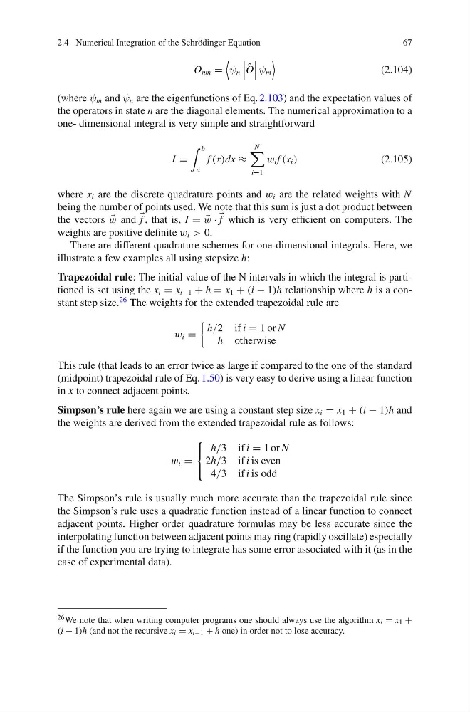
(where ψ m and ψ n are the eigenfunctions of Eq. 2.103) and the expectation values of
the operators in state n are the diagonal elements. The numerical approximation to a
one- dimensional integral is very simple and straightforward
I =
b
a
f (x)dx ≈
N
i=1
w i f (x i )
(2.105)
where x i are the discrete quadrature points and w i are the related weights with N
being the number of points used. We note that this sum is just a dot product between
the vectors
w and
f , that is, I = =
w ·
f which is very efficient on computers. The
weights are positive definite w i > 0.
There are different quadrature schemes for one-dimensional integrals. Here, we
illustrate a few examples all using stepsize h:
Trapezoidal rule: The initial value of the N intervals in which the integral is partitioned is set using the x i = x i−1 + h = x 1 + (i − 1)h relationship where h is a constant step size.
26 The weights for the extended trapezoidal rule are
w i =
h/2 ifi = 1 or N
h otherwise
This rule (that leads to an error twice as large if compared to the one of the standard
(midpoint) trapezoidal rule of Eq. 1.50) is very easy to derive using a linear function
in x to connect adjacent points.
Simpson’s rule here again we are using a constant step size x i = x 1 + (i − 1)h and
the weights are derived from the extended trapezoidal rule as follows:
w i =
⎧
⎨
⎩
h/3 ifi = 1 or N
2h/3 ifi is even
4/3 ifi is odd
The Simpson’s rule is usually much more accurate than the trapezoidal rule since
the Simpson’s rule uses a quadratic function instead of a linear function to connect
adjacent points. Higher order quadrature formulas may be less accurate since the
interpolating function between adjacent points may ring (rapidly oscillate) especially
if the function you are trying to integrate has some error associated with it (as in the
case of experimental data).
26 We note that when writing computer programs one should always use the algorithm x i = x 1 +
(i − 1)h (and not the recursive x i = x i−1 + h one) in order not to lose accuracy.
67
O nm =
ψ n
ˆ
O
ψ m
(2.104)
(where ψ m and ψ n are the eigenfunctions of Eq. 2.103) and the expectation values of
the operators in state n are the diagonal elements. The numerical approximation to a
one- dimensional integral is very simple and straightforward
I =
b
a
f (x)dx ≈
N
i=1
w i f (x i )
(2.105)
where x i are the discrete quadrature points and w i are the related weights with N
being the number of points used. We note that this sum is just a dot product between
the vectors
w and
f , that is, I = =
w ·
f which is very efficient on computers. The
weights are positive definite w i > 0.
There are different quadrature schemes for one-dimensional integrals. Here, we
illustrate a few examples all using stepsize h:
Trapezoidal rule: The initial value of the N intervals in which the integral is partitioned is set using the x i = x i−1 + h = x 1 + (i − 1)h relationship where h is a constant step size.
26 The weights for the extended trapezoidal rule are
w i =
h/2 ifi = 1 or N
h otherwise
This rule (that leads to an error twice as large if compared to the one of the standard
(midpoint) trapezoidal rule of Eq. 1.50) is very easy to derive using a linear function
in x to connect adjacent points.
Simpson’s rule here again we are using a constant step size x i = x 1 + (i − 1)h and
the weights are derived from the extended trapezoidal rule as follows:
w i =
⎧
⎨
⎩
h/3 ifi = 1 or N
2h/3 ifi is even
4/3 ifi is odd
The Simpson’s rule is usually much more accurate than the trapezoidal rule since
the Simpson’s rule uses a quadratic function instead of a linear function to connect
adjacent points. Higher order quadrature formulas may be less accurate since the
interpolating function between adjacent points may ring (rapidly oscillate) especially
if the function you are trying to integrate has some error associated with it (as in the
case of experimental data).
26 We note that when writing computer programs one should always use the algorithm x i = x 1 +
(i − 1)h (and not the recursive x i = x i−1 + h one) in order not to lose accuracy.