

2.3 Realistic Models for Scattering Systems
65
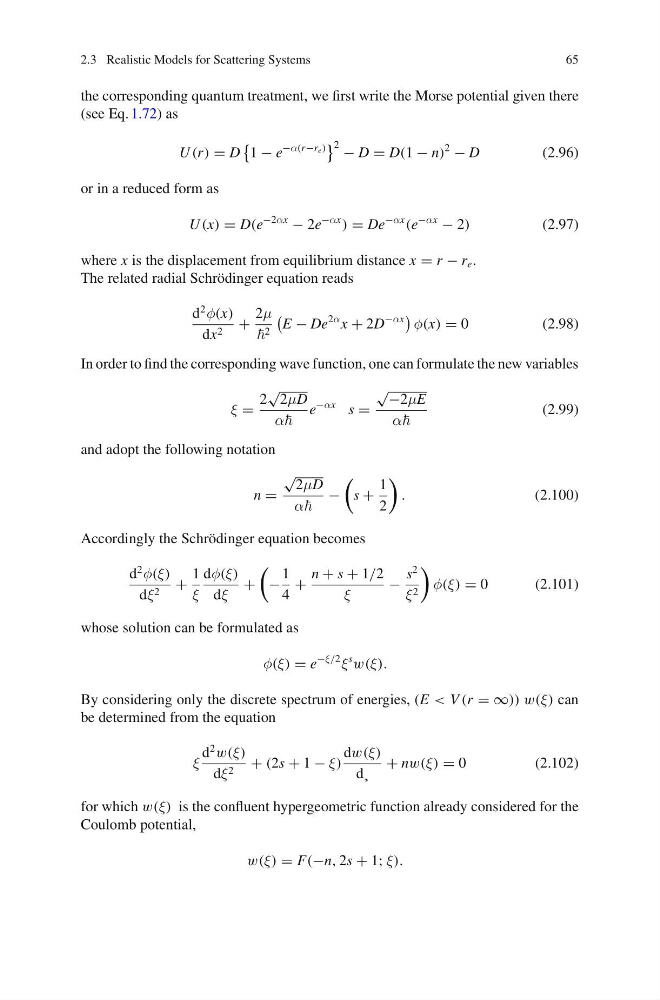
the corresponding quantum treatment, we first write the Morse potential given there
(see Eq. 1.72) as
U (r) = D
1 − e
−α(r−r e )
2 − D = D(1 − n)
2
− D
(2.96)
or in a reduced form as
U (x) = D(e
−2αx
− 2e
−αx
) = De
−αx
(e
−αx
− 2)
(2.97)
where x is the displacement from equilibrium distance x = r − r e .
The related radial Schrödinger equation reads
d
2
φ(x)
dx 2 +
2μ
2
E − De
2α x + 2D
−αx
φ(x) = 0
(2.98)
In order to find the corresponding wave function, one can formulate the new variables
ξ =
2
√
2μD
α
e
−αx s =
√ −2μE
α
(2.99)
and adopt the following notation
n =
√
2μD
α
−
s +
1
2
.
(2.100)
Accordingly the Schrödinger equation becomes
d
2
φ(ξ)
dξ 2 +
1
ξ
dφ(ξ)
dξ
+
−
1
4
+
n + s + 1/2
ξ
−
s
2
ξ 2
φ(ξ) = 0
(2.101)
whose solution can be formulated as
φ(ξ) = e
−ξ/2
ξ
s
w(ξ).
By considering only the discrete spectrum of energies, (E < V (r = ∞)) w(ξ) can
be determined from the equation
ξ
d
2
w(ξ)
dξ 2 + (2s + 1 − ξ)
dw(ξ)
d¸
+ nw(ξ) = 0
(2.102)
for which w(ξ) is the confluent hypergeometric function already considered for the
Coulomb potential,
w(ξ) = F(−n, 2s + 1; ξ).
65
the corresponding quantum treatment, we first write the Morse potential given there
(see Eq. 1.72) as
U (r) = D
1 − e
−α(r−r e )
2 − D = D(1 − n)
2
− D
(2.96)
or in a reduced form as
U (x) = D(e
−2αx
− 2e
−αx
) = De
−αx
(e
−αx
− 2)
(2.97)
where x is the displacement from equilibrium distance x = r − r e .
The related radial Schrödinger equation reads
d
2
φ(x)
dx 2 +
2μ
2
E − De
2α x + 2D
−αx
φ(x) = 0
(2.98)
In order to find the corresponding wave function, one can formulate the new variables
ξ =
2
√
2μD
α
e
−αx s =
√ −2μE
α
(2.99)
and adopt the following notation
n =
√
2μD
α
−
s +
1
2
.
(2.100)
Accordingly the Schrödinger equation becomes
d
2
φ(ξ)
dξ 2 +
1
ξ
dφ(ξ)
dξ
+
−
1
4
+
n + s + 1/2
ξ
−
s
2
ξ 2
φ(ξ) = 0
(2.101)
whose solution can be formulated as
φ(ξ) = e
−ξ/2
ξ
s
w(ξ).
By considering only the discrete spectrum of energies, (E < V (r = ∞)) w(ξ) can
be determined from the equation
ξ
d
2
w(ξ)
dξ 2 + (2s + 1 − ξ)
dw(ξ)
d¸
+ nw(ξ) = 0
(2.102)
for which w(ξ) is the confluent hypergeometric function already considered for the
Coulomb potential,
w(ξ) = F(−n, 2s + 1; ξ).