

60
2 The Quantum Approach to the Two-Body Problem
-25.0
-20.0
-15.0
-10.0
-5.0
0.0
5.0
0
1 0
2 0
3 0
4 0
5 0
6 0
Phase shifts
l
Repulsive potential
Repulsive+Attractive
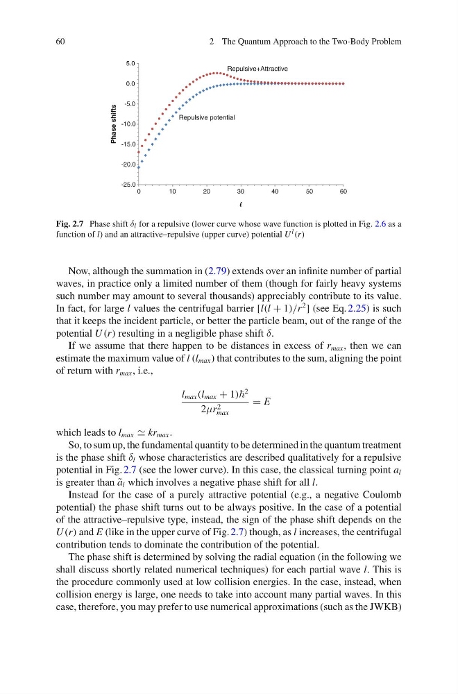
Fig. 2.7 Phase shift δ l for a repulsive (lower curve whose wave function is plotted in Fig. 2.6 as a
function of l) and an attractive–repulsive (upper curve) potential U l (r)
Now, although the summation in (2.79) extends over an infinite number of partial
waves, in practice only a limited number of them (though for fairly heavy systems
such number may amount to several thousands) appreciably contribute to its value.
In fact, for large l values the centrifugal barrier [l(l + 1)/r
2
] (see Eq. 2.25) is such
that it keeps the incident particle, or better the particle beam, out of the range of the
potential U (r) resulting in a negligible phase shift δ.
If we assume that there happen to be distances in excess of r max , then we can
estimate the maximum value of l (l max ) that contributes to the sum, aligning the point
of return with r max , i.e.,
l max (l max + 1)
2
2μr 2
max
= E
which leads to l max kr max .
So, to sum up, the fundamental quantity to be determined in the quantum treatment
is the phase shift δ l whose characteristics are described qualitatively for a repulsive
potential in Fig. 2.7 (see the lower curve). In this case, the classical turning point a l
is greater than ˜
a l which involves a negative phase shift for all l.
Instead for the case of a purely attractive potential (e.g., a negative Coulomb
potential) the phase shift turns out to be always positive. In the case of a potential
of the attractive–repulsive type, instead, the sign of the phase shift depends on the
U (r) and E (like in the upper curve of Fig. 2.7) though, as l increases, the centrifugal
contribution tends to dominate the contribution of the potential.
The phase shift is determined by solving the radial equation (in the following we
shall discuss shortly related numerical techniques) for each partial wave l. This is
the procedure commonly used at low collision energies. In the case, instead, when
collision energy is large, one needs to take into account many partial waves. In this
case, therefore, you may prefer to use numerical approximations (such as the JWKB)
2 The Quantum Approach to the Two-Body Problem
-25.0
-20.0
-15.0
-10.0
-5.0
0.0
5.0
0
1 0
2 0
3 0
4 0
5 0
6 0
Phase shifts
l
Repulsive potential
Repulsive+Attractive
Fig. 2.7 Phase shift δ l for a repulsive (lower curve whose wave function is plotted in Fig. 2.6 as a
function of l) and an attractive–repulsive (upper curve) potential U l (r)
Now, although the summation in (2.79) extends over an infinite number of partial
waves, in practice only a limited number of them (though for fairly heavy systems
such number may amount to several thousands) appreciably contribute to its value.
In fact, for large l values the centrifugal barrier [l(l + 1)/r
2
] (see Eq. 2.25) is such
that it keeps the incident particle, or better the particle beam, out of the range of the
potential U (r) resulting in a negligible phase shift δ.
If we assume that there happen to be distances in excess of r max , then we can
estimate the maximum value of l (l max ) that contributes to the sum, aligning the point
of return with r max , i.e.,
l max (l max + 1)
2
2μr 2
max
= E
which leads to l max kr max .
So, to sum up, the fundamental quantity to be determined in the quantum treatment
is the phase shift δ l whose characteristics are described qualitatively for a repulsive
potential in Fig. 2.7 (see the lower curve). In this case, the classical turning point a l
is greater than ˜
a l which involves a negative phase shift for all l.
Instead for the case of a purely attractive potential (e.g., a negative Coulomb
potential) the phase shift turns out to be always positive. In the case of a potential
of the attractive–repulsive type, instead, the sign of the phase shift depends on the
U (r) and E (like in the upper curve of Fig. 2.7) though, as l increases, the centrifugal
contribution tends to dominate the contribution of the potential.
The phase shift is determined by solving the radial equation (in the following we
shall discuss shortly related numerical techniques) for each partial wave l. This is
the procedure commonly used at low collision energies. In the case, instead, when
collision energy is large, one needs to take into account many partial waves. In this
case, therefore, you may prefer to use numerical approximations (such as the JWKB)