

1.3 The Computation of Scattering Properties
21
tstep is the value of the time step used for the integration
tsup is the maximum time
----------------------------------------------------r = ro
th = acos(-1.) -asin(b/r)
rmass = am1*am2/(am1 + am2)
po = sqrt(2.*rmass*etr)
pr = po*cos(th)
th_dot=po*b/r/r/rmass
time REPEAT FOR GOING FROM 0 TO PAST tsup by tstep
r = r + pr/rmass*tstep
th = th+th_dot*tstep
pr = bˆ2/(rmass* rˆ3) - dpotr(r)
PRINT ’ value of r and theta ’, r, th
IF (r> ro) END
END REPEAT time
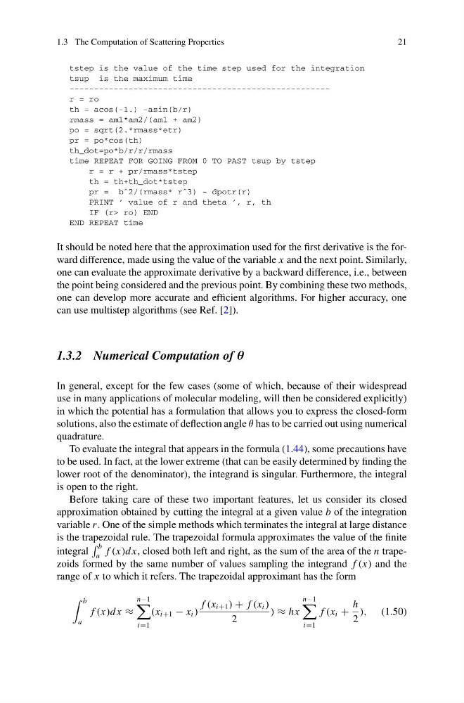
It should be noted here that the approximation used for the first derivative is the forward difference, made using the value of the variable x and the next point. Similarly,
one can evaluate the approximate derivative by a backward difference, i.e., between
the point being considered and the previous point. By combining these two methods,
one can develop more accurate and efficient algorithms. For higher accuracy, one
can use multistep algorithms (see Ref. [2]).
1.3.2 Numerical Computation of θ
In general, except for the few cases (some of which, because of their widespread
use in many applications of molecular modeling, will then be considered explicitly)
in which the potential has a formulation that allows you to express the closed-form
solutions, also the estimate of deflection angle θ has to be carried out using numerical
quadrature.
To evaluate the integral that appears in the formula (1.44), some precautions have
to be used. In fact, at the lower extreme (that can be easily determined by finding the
lower root of the denominator), the integrand is singular. Furthermore, the integral
is open to the right.
Before taking care of these two important features, let us consider its closed
approximation obtained by cutting the integral at a given value b of the integration
variable r . One of the simple methods which terminates the integral at large distance
is the trapezoidal rule. The trapezoidal formula approximates the value of the finite
integral
b
a f (x)dx, closed both left and right, as the sum of the area of the n trapezoids formed by the same number of values sampling the integrand f (x) and the
range of x to which it refers. The trapezoidal approximant has the form
b
a
f (x)dx ≈
n−1
i=1
(x i+1 − x i )
f (x i+1 ) + f (x i )
2
) ≈ hx
n−1
i=1
f (x i +
h
2
), (1.50)
21
tstep is the value of the time step used for the integration
tsup is the maximum time
----------------------------------------------------r = ro
th = acos(-1.) -asin(b/r)
rmass = am1*am2/(am1 + am2)
po = sqrt(2.*rmass*etr)
pr = po*cos(th)
th_dot=po*b/r/r/rmass
time REPEAT FOR GOING FROM 0 TO PAST tsup by tstep
r = r + pr/rmass*tstep
th = th+th_dot*tstep
pr = bˆ2/(rmass* rˆ3) - dpotr(r)
PRINT ’ value of r and theta ’, r, th
IF (r> ro) END
END REPEAT time
It should be noted here that the approximation used for the first derivative is the forward difference, made using the value of the variable x and the next point. Similarly,
one can evaluate the approximate derivative by a backward difference, i.e., between
the point being considered and the previous point. By combining these two methods,
one can develop more accurate and efficient algorithms. For higher accuracy, one
can use multistep algorithms (see Ref. [2]).
1.3.2 Numerical Computation of θ
In general, except for the few cases (some of which, because of their widespread
use in many applications of molecular modeling, will then be considered explicitly)
in which the potential has a formulation that allows you to express the closed-form
solutions, also the estimate of deflection angle θ has to be carried out using numerical
quadrature.
To evaluate the integral that appears in the formula (1.44), some precautions have
to be used. In fact, at the lower extreme (that can be easily determined by finding the
lower root of the denominator), the integrand is singular. Furthermore, the integral
is open to the right.
Before taking care of these two important features, let us consider its closed
approximation obtained by cutting the integral at a given value b of the integration
variable r . One of the simple methods which terminates the integral at large distance
is the trapezoidal rule. The trapezoidal formula approximates the value of the finite
integral
b
a f (x)dx, closed both left and right, as the sum of the area of the n trapezoids formed by the same number of values sampling the integrand f (x) and the
range of x to which it refers. The trapezoidal approximant has the form
b
a
f (x)dx ≈
n−1
i=1
(x i+1 − x i )
f (x i+1 ) + f (x i )
2
) ≈ hx
n−1
i=1
f (x i +
h
2
), (1.50)