

1.2 Classical Mechanics of Two-Particle Collisions
17
-10.0
-5.0
0.0
5.0
10.0
-10.0
-5.0
0.0
5.0
10.0
orbiting
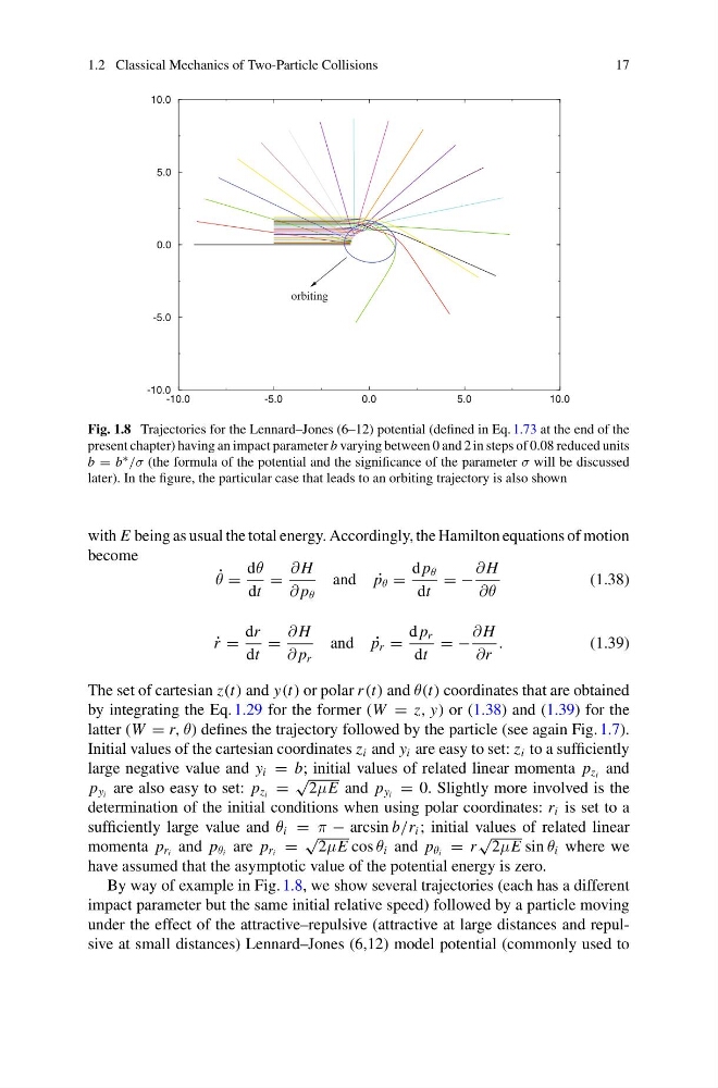
Fig. 1.8 Trajectories for the Lennard–Jones (6–12) potential (defined in Eq. 1.73 at the end of the
present chapter) having an impact parameter b varying between 0 and 2 in steps of 0.08 reduced units
b = b ∗ /σ (the formula of the potential and the significance of the parameter σ will be discussed
later). In the figure, the particular case that leads to an orbiting trajectory is also shown
with E being as usual the total energy. Accordingly, the Hamilton equations of motion
become
˙
θ =
dθ
dt
=
∂ H
∂ p θ
and ˙
p θ =
d p θ
dt
= −
∂ H
∂θ
(1.38)
˙
r =
dr
dt
=
∂ H
∂ p r
and ˙
p r =
d p r
dt
= −
∂ H
∂r
.
(1.39)
The set of cartesian z(t) and y(t) or polar r (t) and θ(t) coordinates that are obtained
by integrating the Eq. 1.29 for the former (W = z, y) or (1.38) and (1.39) for the
latter (W = r, θ) defines the trajectory followed by the particle (see again Fig. 1.7).
Initial values of the cartesian coordinates z i and y i are easy to set: z i to a sufficiently
large negative value and y i = b; initial values of related linear momenta p z i and
p y i are also easy to set: p z i =
√
2μE and p y i = 0. Slightly more involved is the
determination of the initial conditions when using polar coordinates: r i is set to a
sufficiently large value and θ i = π − arcsin b/r i ; initial values of related linear
momenta p r i and p θ i are p r i =
√
2μE cos θ i and p θ i = r
√
2μE sin θ i where we
have assumed that the asymptotic value of the potential energy is zero.
By way of example in Fig. 1.8, we show several trajectories (each has a different
impact parameter but the same initial relative speed) followed by a particle moving
under the effect of the attractive–repulsive (attractive at large distances and repulsive at small distances) Lennard–Jones (6,12) model potential (commonly used to
17
-10.0
-5.0
0.0
5.0
10.0
-10.0
-5.0
0.0
5.0
10.0
orbiting
Fig. 1.8 Trajectories for the Lennard–Jones (6–12) potential (defined in Eq. 1.73 at the end of the
present chapter) having an impact parameter b varying between 0 and 2 in steps of 0.08 reduced units
b = b ∗ /σ (the formula of the potential and the significance of the parameter σ will be discussed
later). In the figure, the particular case that leads to an orbiting trajectory is also shown
with E being as usual the total energy. Accordingly, the Hamilton equations of motion
become
˙
θ =
dθ
dt
=
∂ H
∂ p θ
and ˙
p θ =
d p θ
dt
= −
∂ H
∂θ
(1.38)
˙
r =
dr
dt
=
∂ H
∂ p r
and ˙
p r =
d p r
dt
= −
∂ H
∂r
.
(1.39)
The set of cartesian z(t) and y(t) or polar r (t) and θ(t) coordinates that are obtained
by integrating the Eq. 1.29 for the former (W = z, y) or (1.38) and (1.39) for the
latter (W = r, θ) defines the trajectory followed by the particle (see again Fig. 1.7).
Initial values of the cartesian coordinates z i and y i are easy to set: z i to a sufficiently
large negative value and y i = b; initial values of related linear momenta p z i and
p y i are also easy to set: p z i =
√
2μE and p y i = 0. Slightly more involved is the
determination of the initial conditions when using polar coordinates: r i is set to a
sufficiently large value and θ i = π − arcsin b/r i ; initial values of related linear
momenta p r i and p θ i are p r i =
√
2μE cos θ i and p θ i = r
√
2μE sin θ i where we
have assumed that the asymptotic value of the potential energy is zero.
By way of example in Fig. 1.8, we show several trajectories (each has a different
impact parameter but the same initial relative speed) followed by a particle moving
under the effect of the attractive–repulsive (attractive at large distances and repulsive at small distances) Lennard–Jones (6,12) model potential (commonly used to