

4.3 Beyond Full Quantum Calculations
129
spatial probability density remains unchanged. Typically, there is no eigenstate of
the final Hamiltonian with the same functional form as the initial state. The system
ends in a linear combination of states that sum to reproduce the initial probability
density.
In the adiabatic scheme, conditions are considered to change gradually. Accordingly, the system is allowed to adapt its configuration during the process, hence the
probability density is modified by the process. Typically, the system starts in an
eigenstate of the initial Hamiltonian, it will end in the corresponding eigenstate of
the final Hamiltonian
Of the first type is the popular infinite order sudden approximation (IOSA) that
applies, at the same time, an energy and a centrifugal sudden dimensionality reduction to the full three-dimensional Eq. (4.26) formulation of the scattering equations.
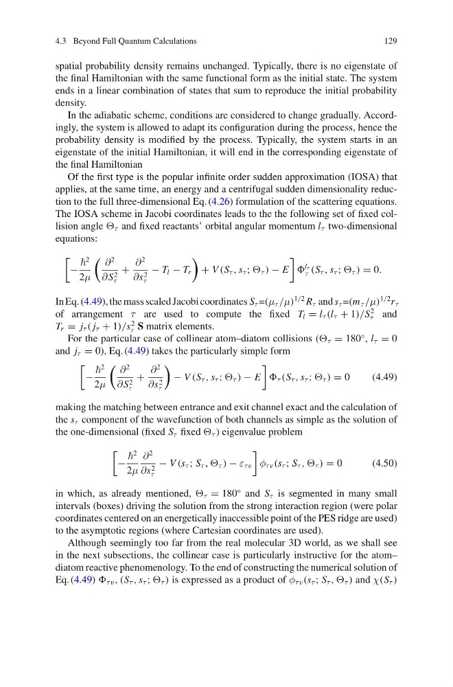
The IOSA scheme in Jacobi coordinates leads to the the following set of fixed collision angle τ and fixed reactants’ orbital angular momentum l τ two-dimensional
equations:
−
2
2μ
∂
2
∂ S 2
τ
+
∂
2
∂s 2
τ
− T l − T r
+ V (S τ , s τ ; τ ) − E
l τ
τ (S τ , s τ ; τ ) = 0.
In Eq. (4.49), the mass scaled Jacobi coordinates S τ =(μ τ /μ)
1/2 R τ and s τ =(m τ /μ)
1/2 r τ
of arrangement τ are used to compute the fixed T l = l τ (l τ + 1)/S
2
τ and
T r = j τ ( j τ + 1)/s
2
τ S matrix elements.
For the particular case of collinear atom–diatom collisions ( τ = 180
◦ , l τ = 0
and j τ = 0), Eq. (4.49) takes the particularly simple form
−
2
2μ
∂
2
∂ S 2
τ
+
∂
2
∂s 2
τ
− V (S τ , s τ ; τ ) − E
τ (S τ , s τ ; τ ) = 0
(4.49)
making the matching between entrance and exit channel exact and the calculation of
the s τ component of the wavefunction of both channels as simple as the solution of
the one-dimensional (fixed S τ fixed τ ) eigenvalue problem
−
2
2μ
∂
2
∂s 2
τ
− V (s τ ; S τ , , τ ) − ε τ v
φ τ v (s τ ; S τ , , τ ) = 0
(4.50)
in which, as already mentioned, τ = 180
◦ and S τ is segmented in many small
intervals (boxes) driving the solution from the strong interaction region (were polar
coordinates centered on an energetically inaccessible point of the PES ridge are used)
to the asymptotic regions (where Cartesian coordinates are used).
Although seemingly too far from the real molecular 3D world, as we shall see
in the next subsections, the collinear case is particularly instructive for the atom–
diatom reactive phenomenology. To the end of constructing the numerical solution of
Eq. (4.49) τ v , (S τ , s τ ; τ ) is expressed as a product of φ τ v (s τ ; S τ , , τ ) and χ(S τ )
129
spatial probability density remains unchanged. Typically, there is no eigenstate of
the final Hamiltonian with the same functional form as the initial state. The system
ends in a linear combination of states that sum to reproduce the initial probability
density.
In the adiabatic scheme, conditions are considered to change gradually. Accordingly, the system is allowed to adapt its configuration during the process, hence the
probability density is modified by the process. Typically, the system starts in an
eigenstate of the initial Hamiltonian, it will end in the corresponding eigenstate of
the final Hamiltonian
Of the first type is the popular infinite order sudden approximation (IOSA) that
applies, at the same time, an energy and a centrifugal sudden dimensionality reduction to the full three-dimensional Eq. (4.26) formulation of the scattering equations.
The IOSA scheme in Jacobi coordinates leads to the the following set of fixed collision angle τ and fixed reactants’ orbital angular momentum l τ two-dimensional
equations:
−
2
2μ
∂
2
∂ S 2
τ
+
∂
2
∂s 2
τ
− T l − T r
+ V (S τ , s τ ; τ ) − E
l τ
τ (S τ , s τ ; τ ) = 0.
In Eq. (4.49), the mass scaled Jacobi coordinates S τ =(μ τ /μ)
1/2 R τ and s τ =(m τ /μ)
1/2 r τ
of arrangement τ are used to compute the fixed T l = l τ (l τ + 1)/S
2
τ and
T r = j τ ( j τ + 1)/s
2
τ S matrix elements.
For the particular case of collinear atom–diatom collisions ( τ = 180
◦ , l τ = 0
and j τ = 0), Eq. (4.49) takes the particularly simple form
−
2
2μ
∂
2
∂ S 2
τ
+
∂
2
∂s 2
τ
− V (S τ , s τ ; τ ) − E
τ (S τ , s τ ; τ ) = 0
(4.49)
making the matching between entrance and exit channel exact and the calculation of
the s τ component of the wavefunction of both channels as simple as the solution of
the one-dimensional (fixed S τ fixed τ ) eigenvalue problem
−
2
2μ
∂
2
∂s 2
τ
− V (s τ ; S τ , , τ ) − ε τ v
φ τ v (s τ ; S τ , , τ ) = 0
(4.50)
in which, as already mentioned, τ = 180
◦ and S τ is segmented in many small
intervals (boxes) driving the solution from the strong interaction region (were polar
coordinates centered on an energetically inaccessible point of the PES ridge are used)
to the asymptotic regions (where Cartesian coordinates are used).
Although seemingly too far from the real molecular 3D world, as we shall see
in the next subsections, the collinear case is particularly instructive for the atom–
diatom reactive phenomenology. To the end of constructing the numerical solution of
Eq. (4.49) τ v , (S τ , s τ ; τ ) is expressed as a product of φ τ v (s τ ; S τ , , τ ) and χ(S τ )