

4.1 The Combined Dynamics of Electrons and Nuclei
115
of the electrons from the motion of the nuclei (which is justified by the fact that the
motion of electrons is much faster than that of the nuclei which allows them to redistribute almost instantaneously around the nuclei in motion). The Born–Oppenheimer
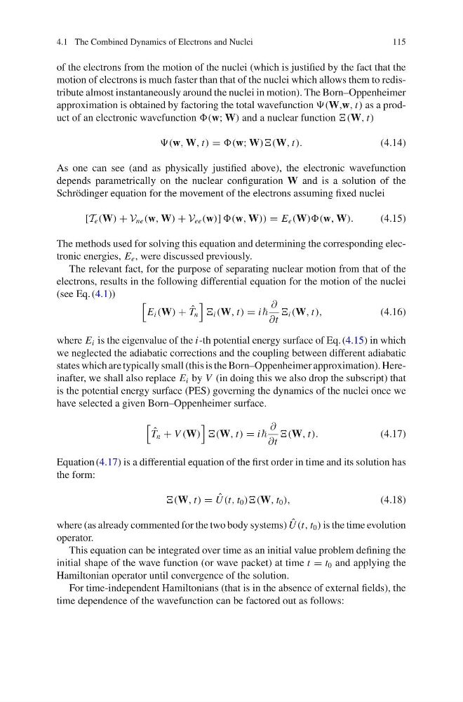
approximation is obtained by factoring the total wavefunction (W,w, t) as a product of an electronic wavefunction (w; W) and a nuclear function (W, t)
(w, W, t) = (w; W))(W, t).
(4.14)
As one can see (and as physically justified above), the electronic wavefunction
depends parametrically on the nuclear configuration W and is a solution of the
Schrödinger equation for the movement of the electrons assuming fixed nuclei
[T e (W) + V ne (w, W) + V ee (w)] (w, W)) = E e (W))(w, W).
(4.15)
The methods used for solving this equation and determining the corresponding electronic energies, E e , were discussed previously.
The relevant fact, for the purpose of separating nuclear motion from that of the
electrons, results in the following differential equation for the motion of the nuclei
(see Eq. (4.1))
E i (W) + ˆ
T n
i (W, t) = i
∂
∂t
i (W, t),
(4.16)
where E i is the eigenvalue of the i-th potential energy surface of Eq. (4.15) in which
we neglected the adiabatic corrections and the coupling between different adiabatic
states which are typically small (this is the Born–Oppenheimer approximation). Hereinafter, we shall also replace E i by V (in doing this we also drop the subscript) that
is the potential energy surface (PES) governing the dynamics of the nuclei once we
have selected a given Born–Oppenheimer surface.
ˆ
T n + V (W)
(W, t) = i
∂
∂t
(W, t).
(4.17)
Equation (4.17) is a differential equation of the first order in time and its solution has
the form:
(W, t) = ˆ
U (t, t 0 ))(W, t 0 ),
(4.18)
where (as already commented for the two body systems) ˆ
U (t, t 0 ) is the time evolution
operator.
This equation can be integrated over time as an initial value problem defining the
initial shape of the wave function (or wave packet) at time t = t 0 and applying the
Hamiltonian operator until convergence of the solution.
For time-independent Hamiltonians (that is in the absence of external fields), the
time dependence of the wavefunction can be factored out as follows:
115
of the electrons from the motion of the nuclei (which is justified by the fact that the
motion of electrons is much faster than that of the nuclei which allows them to redistribute almost instantaneously around the nuclei in motion). The Born–Oppenheimer
approximation is obtained by factoring the total wavefunction (W,w, t) as a product of an electronic wavefunction (w; W) and a nuclear function (W, t)
(w, W, t) = (w; W))(W, t).
(4.14)
As one can see (and as physically justified above), the electronic wavefunction
depends parametrically on the nuclear configuration W and is a solution of the
Schrödinger equation for the movement of the electrons assuming fixed nuclei
[T e (W) + V ne (w, W) + V ee (w)] (w, W)) = E e (W))(w, W).
(4.15)
The methods used for solving this equation and determining the corresponding electronic energies, E e , were discussed previously.
The relevant fact, for the purpose of separating nuclear motion from that of the
electrons, results in the following differential equation for the motion of the nuclei
(see Eq. (4.1))
E i (W) + ˆ
T n
i (W, t) = i
∂
∂t
i (W, t),
(4.16)
where E i is the eigenvalue of the i-th potential energy surface of Eq. (4.15) in which
we neglected the adiabatic corrections and the coupling between different adiabatic
states which are typically small (this is the Born–Oppenheimer approximation). Hereinafter, we shall also replace E i by V (in doing this we also drop the subscript) that
is the potential energy surface (PES) governing the dynamics of the nuclei once we
have selected a given Born–Oppenheimer surface.
ˆ
T n + V (W)
(W, t) = i
∂
∂t
(W, t).
(4.17)
Equation (4.17) is a differential equation of the first order in time and its solution has
the form:
(W, t) = ˆ
U (t, t 0 ))(W, t 0 ),
(4.18)
where (as already commented for the two body systems) ˆ
U (t, t 0 ) is the time evolution
operator.
This equation can be integrated over time as an initial value problem defining the
initial shape of the wave function (or wave packet) at time t = t 0 and applying the
Hamiltonian operator until convergence of the solution.
For time-independent Hamiltonians (that is in the absence of external fields), the
time dependence of the wavefunction can be factored out as follows: