

3.3 Toward Extended Applications
95
3.3 Toward Extended Applications
3.3.1 Computation of Other Molecular Properties
As you have already seen in Chap. 2, the energies of the orbitals and the coefficients
of the expansion of molecular orbitals into atomic orbitals obtained by solving the
Schrödinger equation can be used to compute other properties of the investigated
system. In other words, one can evaluate the physical observables associated with a
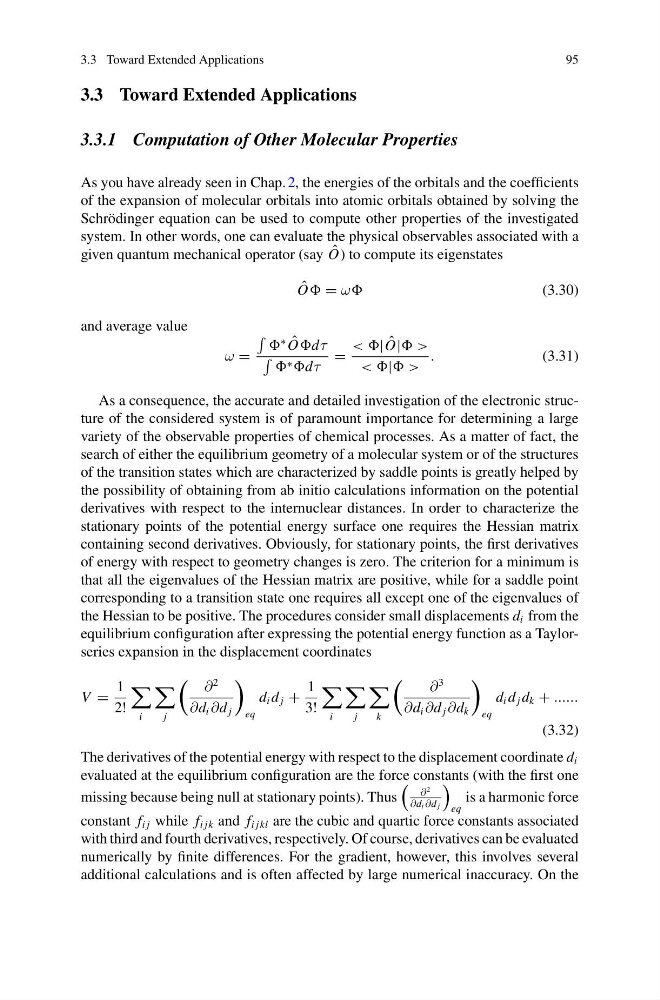
given quantum mechanical operator (say ˆ
O) to compute its eigenstates
ˆ
O = ω
(3.30)
and average value
ω =
∗ ˆ
Odτ
∗ dτ
=
< <| ˆ
O| >
< <| >
.
(3.31)
As a consequence, the accurate and detailed investigation of the electronic structure of the considered system is of paramount importance for determining a large
variety of the observable properties of chemical processes. As a matter of fact, the
search of either the equilibrium geometry of a molecular system or of the structures
of the transition states which are characterized by saddle points is greatly helped by
the possibility of obtaining from ab initio calculations information on the potential
derivatives with respect to the internuclear distances. In order to characterize the
stationary points of the potential energy surface one requires the Hessian matrix
containing second derivatives. Obviously, for stationary points, the first derivatives
of energy with respect to geometry changes is zero. The criterion for a minimum is
that all the eigenvalues of the Hessian matrix are positive, while for a saddle point
corresponding to a transition state one requires all except one of the eigenvalues of
the Hessian to be positive. The procedures consider small displacements d i from the
equilibrium configuration after expressing the potential energy function as a Taylorseries expansion in the displacement coordinates
V =
1
2!
i
j
∂
2
∂d i ∂d j
eq
d i d j +
1
3!
i
j
k
∂
3
∂d i ∂d j ∂d k
eq
d i d j d k + ......
(3.32)
The derivatives of the potential energy with respect to the displacement coordinate d i
evaluated at the equilibrium configuration are the force constants (with the first one
missing because being null at stationary points). Thus
∂
2
∂d i ∂d j
eq
is a harmonic force
constant f i j while f i jk and f i jkl are the cubic and quartic force constants associated
with third and fourth derivatives, respectively. Of course, derivatives can be evaluated
numerically by finite differences. For the gradient, however, this involves several
additional calculations and is often affected by large numerical inaccuracy. On the
95
3.3 Toward Extended Applications
3.3.1 Computation of Other Molecular Properties
As you have already seen in Chap. 2, the energies of the orbitals and the coefficients
of the expansion of molecular orbitals into atomic orbitals obtained by solving the
Schrödinger equation can be used to compute other properties of the investigated
system. In other words, one can evaluate the physical observables associated with a
given quantum mechanical operator (say ˆ
O) to compute its eigenstates
ˆ
O = ω
(3.30)
and average value
ω =
∗ ˆ
Odτ
∗ dτ
=
< <| ˆ
O| >
< <| >
.
(3.31)
As a consequence, the accurate and detailed investigation of the electronic structure of the considered system is of paramount importance for determining a large
variety of the observable properties of chemical processes. As a matter of fact, the
search of either the equilibrium geometry of a molecular system or of the structures
of the transition states which are characterized by saddle points is greatly helped by
the possibility of obtaining from ab initio calculations information on the potential
derivatives with respect to the internuclear distances. In order to characterize the
stationary points of the potential energy surface one requires the Hessian matrix
containing second derivatives. Obviously, for stationary points, the first derivatives
of energy with respect to geometry changes is zero. The criterion for a minimum is
that all the eigenvalues of the Hessian matrix are positive, while for a saddle point
corresponding to a transition state one requires all except one of the eigenvalues of
the Hessian to be positive. The procedures consider small displacements d i from the
equilibrium configuration after expressing the potential energy function as a Taylorseries expansion in the displacement coordinates
V =
1
2!
i
j
∂
2
∂d i ∂d j
eq
d i d j +
1
3!
i
j
k
∂
3
∂d i ∂d j ∂d k
eq
d i d j d k + ......
(3.32)
The derivatives of the potential energy with respect to the displacement coordinate d i
evaluated at the equilibrium configuration are the force constants (with the first one
missing because being null at stationary points). Thus
∂
2
∂d i ∂d j
eq
is a harmonic force
constant f i j while f i jk and f i jkl are the cubic and quartic force constants associated
with third and fourth derivatives, respectively. Of course, derivatives can be evaluated
numerically by finite differences. For the gradient, however, this involves several
additional calculations and is often affected by large numerical inaccuracy. On the