

3.2 Model Spin Hamiltonians for Isotropic Interactions
77
These eigenstates share the common feature that at least one of the local M S values
is not equal to ±M max
S . For example the Ising eigenstates in Fig. 3.6 with energy J
have either on the left or the right (or both) centers an αβ determinant. As soon as
one adds the spatial part to the wave function, these determinants are raised in energy
since they lack the stabilization by the exchange integral K present in the energy
expression of the |αα| and |ββ| determinants. Consequently, in any practical application focused on magnetic interactions one should only consider the eigenstates of
the Ising Hamiltonian with M S = 0orM max
S .
3.3 From Micro to Macro: The Bottom-Up Approach
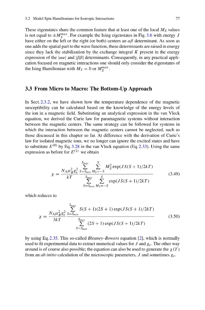
In Sect. 2.3.2, we have shown how the temperature dependence of the magnetic
susceptibility can be calculated based on the knowledge of the energy levels of
the ion in a magnetic field. Substituting an analytical expression in the van Vleck
equation, we derived the Curie law for paramagnetic systems without interaction
between the magnetic centers. The same strategy can be followed for systems in
which the interaction between the magnetic centers cannot be neglected, such as
those discussed in this chapter so far. At difference with the derivation of Curie’s
law for isolated magnetic ions, we no longer can ignore the excited states and have
to substitute E (0) by Eq. 3.28 in the van Vleck equation (Eq. 2.33). Using the same
expression as before for E (1) we obtain
χ =
N A µ 2
B g 2
e
kT
S max
S=S min
S
M S =−S
M 2
S exp(JS(S + 1)/2kT)
S max
S=S min
S
M S =−S
exp(JS(S + 1)/2kT)
(3.49)
which reduces to
χ =
N A µ 2
B g 2
e
3kT
S max
S=S min
S(S + 1)(2S + 1) exp(JS(S + 1)/2kT)
S max
S=S min
(2S + 1) exp(JS(S + 1)/2kT)
(3.50)
by using Eq. 2.35. This so-called Bleaney–Bowers equation [2], which is normally
used to fit experimental data to extract numerical values for J and g e . The other way
around is of course also possible; the equation can also be used to generate the χ(T )
from an ab initio calculation of the microscopic parameters, J and sometimes g e .
77
These eigenstates share the common feature that at least one of the local M S values
is not equal to ±M max
S . For example the Ising eigenstates in Fig. 3.6 with energy J
have either on the left or the right (or both) centers an αβ determinant. As soon as
one adds the spatial part to the wave function, these determinants are raised in energy
since they lack the stabilization by the exchange integral K present in the energy
expression of the |αα| and |ββ| determinants. Consequently, in any practical application focused on magnetic interactions one should only consider the eigenstates of
the Ising Hamiltonian with M S = 0orM max
S .
3.3 From Micro to Macro: The Bottom-Up Approach
In Sect. 2.3.2, we have shown how the temperature dependence of the magnetic
susceptibility can be calculated based on the knowledge of the energy levels of
the ion in a magnetic field. Substituting an analytical expression in the van Vleck
equation, we derived the Curie law for paramagnetic systems without interaction
between the magnetic centers. The same strategy can be followed for systems in
which the interaction between the magnetic centers cannot be neglected, such as
those discussed in this chapter so far. At difference with the derivation of Curie’s
law for isolated magnetic ions, we no longer can ignore the excited states and have
to substitute E (0) by Eq. 3.28 in the van Vleck equation (Eq. 2.33). Using the same
expression as before for E (1) we obtain
χ =
N A µ 2
B g 2
e
kT
S max
S=S min
S
M S =−S
M 2
S exp(JS(S + 1)/2kT)
S max
S=S min
S
M S =−S
exp(JS(S + 1)/2kT)
(3.49)
which reduces to
χ =
N A µ 2
B g 2
e
3kT
S max
S=S min
S(S + 1)(2S + 1) exp(JS(S + 1)/2kT)
S max
S=S min
(2S + 1) exp(JS(S + 1)/2kT)
(3.50)
by using Eq. 2.35. This so-called Bleaney–Bowers equation [2], which is normally
used to fit experimental data to extract numerical values for J and g e . The other way
around is of course also possible; the equation can also be used to generate the χ(T )
from an ab initio calculation of the microscopic parameters, J and sometimes g e .