

3.2 Model Spin Hamiltonians for Isotropic Interactions
69
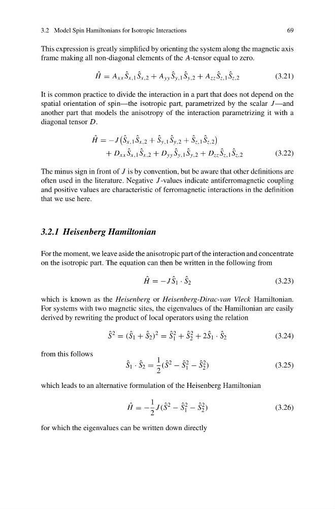
This expression is greatly simplified by orienting the system along the magnetic axis
frame making all non-diagonal elements of the A-tensor equal to zero.
ˆ
H = A xx ˆ
S x,1 ˆ
S x,2 + A yy ˆ
S y,1 ˆ
S y,2 + A zz ˆ
S z,1 ˆ
S z,2
(3.21)
It is common practice to divide the interaction in a part that does not depend on the
spatial orientation of spin—the isotropic part, parametrized by the scalar J —and
another part that models the anisotropy of the interaction parametrizing it with a
diagonal tensor D.
ˆ
H =−J
ˆ
S x,1 ˆ
S x,2 + ˆ
S y,1 ˆ
S y,2 + ˆ
S z,1 ˆ
S z,2
+ D xx ˆ
S x,1 ˆ
S x,2 + D yy ˆ
S y,1 ˆ
S y,2 + D zz ˆ
S z,1 ˆ
S z,2
(3.22)
The minus sign in front of J is by convention, but be aware that other definitions are
often used in the literature. Negative J -values indicate antiferromagnetic coupling
and positive values are characteristic of ferromagnetic interactions in the definition
that we use here.
3.2.1 Heisenberg Hamiltonian
For the moment, we leave aside the anisotropic part of the interaction and concentrate
on the isotropic part. The equation can then be written in the following from
ˆ
H =−J ˆ
S 1 · ˆ
S 2
(3.23)
which is known as the Heisenberg or Heisenberg-Dirac-van Vleck Hamiltonian.
For systems with two magnetic sites, the eigenvalues of the Hamiltonian are easily
derived by rewriting the product of local operators using the relation
ˆ
S
2 = ( ˆ
S 1 + ˆ
S 2 )
2 = ˆ
S
2
1 + ˆ
S
2
2 + 2 ˆ
S 1 · ˆ
S 2
(3.24)
from this follows
ˆ
S 1 · ˆ
S 2 =
1
2
( ˆ
S
2 − ˆ
S
2
1 − ˆ
S
2
2 )
(3.25)
which leads to an alternative formulation of the Heisenberg Hamiltonian
ˆ
H =−
1
2
J ( ˆ
S
2 − ˆ
S
2
1 − ˆ
S
2
2 )
(3.26)
for which the eigenvalues can be written down directly
69
This expression is greatly simplified by orienting the system along the magnetic axis
frame making all non-diagonal elements of the A-tensor equal to zero.
ˆ
H = A xx ˆ
S x,1 ˆ
S x,2 + A yy ˆ
S y,1 ˆ
S y,2 + A zz ˆ
S z,1 ˆ
S z,2
(3.21)
It is common practice to divide the interaction in a part that does not depend on the
spatial orientation of spin—the isotropic part, parametrized by the scalar J —and
another part that models the anisotropy of the interaction parametrizing it with a
diagonal tensor D.
ˆ
H =−J
ˆ
S x,1 ˆ
S x,2 + ˆ
S y,1 ˆ
S y,2 + ˆ
S z,1 ˆ
S z,2
+ D xx ˆ
S x,1 ˆ
S x,2 + D yy ˆ
S y,1 ˆ
S y,2 + D zz ˆ
S z,1 ˆ
S z,2
(3.22)
The minus sign in front of J is by convention, but be aware that other definitions are
often used in the literature. Negative J -values indicate antiferromagnetic coupling
and positive values are characteristic of ferromagnetic interactions in the definition
that we use here.
3.2.1 Heisenberg Hamiltonian
For the moment, we leave aside the anisotropic part of the interaction and concentrate
on the isotropic part. The equation can then be written in the following from
ˆ
H =−J ˆ
S 1 · ˆ
S 2
(3.23)
which is known as the Heisenberg or Heisenberg-Dirac-van Vleck Hamiltonian.
For systems with two magnetic sites, the eigenvalues of the Hamiltonian are easily
derived by rewriting the product of local operators using the relation
ˆ
S
2 = ( ˆ
S 1 + ˆ
S 2 )
2 = ˆ
S
2
1 + ˆ
S
2
2 + 2 ˆ
S 1 · ˆ
S 2
(3.24)
from this follows
ˆ
S 1 · ˆ
S 2 =
1
2
( ˆ
S
2 − ˆ
S
2
1 − ˆ
S
2
2 )
(3.25)
which leads to an alternative formulation of the Heisenberg Hamiltonian
ˆ
H =−
1
2
J ( ˆ
S
2 − ˆ
S
2
1 − ˆ
S
2
2 )
(3.26)
for which the eigenvalues can be written down directly