

3.1 Localized Versus Delocalized Description of the Two-Electron/Two-Orbital Problem
67
singlet wave function shown earlier in Eqs. 3.7 and 3.16. Instead of introducing an
extra variational freedom by adding ionic contributions with optimized weight, the
extra freedom is now obtained by allowing the localized orbitals to be mutually
nonorthogonal and optimizing their overlap. Not surprisingly, we get no additional
improvement if we now include ionic terms, so this VB approach with nonorthogonal
orbitals gives no improvement as compared to the VB approach with orthogonal
orbitals and ionic terms, but the nonorthogonal VB approach does allow us to write
the singlet wave function Ψ(0, 0) in terms of a covalent contribution alone.
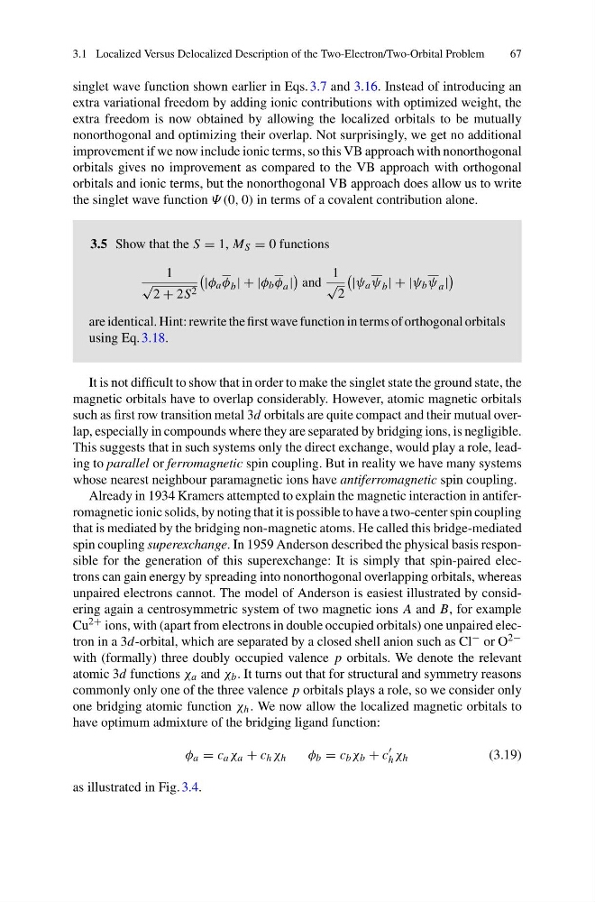
3.5 Show that the S = 1, M S = 0 functions
1
√
2 + 2S 2
|φ a φ b |+|φ b φ a |
and
1
√
2
|ψ a ψ b |+|ψ b ψ a |
are identical. Hint: rewrite the first wave function in terms of orthogonal orbitals
using Eq. 3.18.
It is not difficult to show that in order to make the singlet state the ground state, the
magnetic orbitals have to overlap considerably. However, atomic magnetic orbitals
such as first row transition metal 3d orbitals are quite compact and their mutual overlap, especially in compounds where they are separated by bridging ions, is negligible.
This suggests that in such systems only the direct exchange, would play a role, leading to parallel or ferromagnetic spin coupling. But in reality we have many systems
whose nearest neighbour paramagnetic ions have antiferromagnetic spin coupling.
Already in 1934 Kramers attempted to explain the magnetic interaction in antiferromagnetic ionic solids, by noting that it is possible to have a two-center spin coupling
that is mediated by the bridging non-magnetic atoms. He called this bridge-mediated
spin coupling superexchange. In 1959 Anderson described the physical basis responsible for the generation of this superexchange: It is simply that spin-paired electrons can gain energy by spreading into nonorthogonal overlapping orbitals, whereas
unpaired electrons cannot. The model of Anderson is easiest illustrated by considering again a centrosymmetric system of two magnetic ions A and B, for example
Cu 2+ ions, with (apart from electrons in double occupied orbitals) one unpaired electron in a 3d-orbital, which are separated by a closed shell anion such as Cl − or O 2−
with (formally) three doubly occupied valence p orbitals. We denote the relevant
atomic 3d functions χ a and χ b . It turns out that for structural and symmetry reasons
commonly only one of the three valence p orbitals plays a role, so we consider only
one bridging atomic function χ h . We now allow the localized magnetic orbitals to
have optimum admixture of the bridging ligand function:
φ a = c a χ a + c h χ h
φ b = c b χ b + c
′
h χ h
(3.19)
as illustrated in Fig. 3.4.
67
singlet wave function shown earlier in Eqs. 3.7 and 3.16. Instead of introducing an
extra variational freedom by adding ionic contributions with optimized weight, the
extra freedom is now obtained by allowing the localized orbitals to be mutually
nonorthogonal and optimizing their overlap. Not surprisingly, we get no additional
improvement if we now include ionic terms, so this VB approach with nonorthogonal
orbitals gives no improvement as compared to the VB approach with orthogonal
orbitals and ionic terms, but the nonorthogonal VB approach does allow us to write
the singlet wave function Ψ(0, 0) in terms of a covalent contribution alone.
3.5 Show that the S = 1, M S = 0 functions
1
√
2 + 2S 2
|φ a φ b |+|φ b φ a |
and
1
√
2
|ψ a ψ b |+|ψ b ψ a |
are identical. Hint: rewrite the first wave function in terms of orthogonal orbitals
using Eq. 3.18.
It is not difficult to show that in order to make the singlet state the ground state, the
magnetic orbitals have to overlap considerably. However, atomic magnetic orbitals
such as first row transition metal 3d orbitals are quite compact and their mutual overlap, especially in compounds where they are separated by bridging ions, is negligible.
This suggests that in such systems only the direct exchange, would play a role, leading to parallel or ferromagnetic spin coupling. But in reality we have many systems
whose nearest neighbour paramagnetic ions have antiferromagnetic spin coupling.
Already in 1934 Kramers attempted to explain the magnetic interaction in antiferromagnetic ionic solids, by noting that it is possible to have a two-center spin coupling
that is mediated by the bridging non-magnetic atoms. He called this bridge-mediated
spin coupling superexchange. In 1959 Anderson described the physical basis responsible for the generation of this superexchange: It is simply that spin-paired electrons can gain energy by spreading into nonorthogonal overlapping orbitals, whereas
unpaired electrons cannot. The model of Anderson is easiest illustrated by considering again a centrosymmetric system of two magnetic ions A and B, for example
Cu 2+ ions, with (apart from electrons in double occupied orbitals) one unpaired electron in a 3d-orbital, which are separated by a closed shell anion such as Cl − or O 2−
with (formally) three doubly occupied valence p orbitals. We denote the relevant
atomic 3d functions χ a and χ b . It turns out that for structural and symmetry reasons
commonly only one of the three valence p orbitals plays a role, so we consider only
one bridging atomic function χ h . We now allow the localized magnetic orbitals to
have optimum admixture of the bridging ligand function:
φ a = c a χ a + c h χ h
φ b = c b χ b + c
′
h χ h
(3.19)
as illustrated in Fig. 3.4.