

48
2 One Magnetic Center
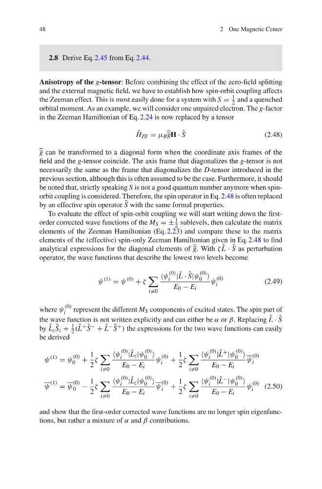
2.8 Derive Eq. 2.45 from Eq. 2.44.
Anisotropy of the g-tensor: Before combining the effect of the zero-field splitting
and the external magnetic field, we have to establish how spin-orbit coupling affects
the Zeeman effect. This is most easily done for a system with S =
1
2 and a quenched
orbital moment. As an example, we will consider one unpaired electron. The g-factor
in the Zeeman Hamiltonian of Eq. 2.24 is now replaced by a tensor
ˆ
H ZE = μ B gH · ˆ
S
(2.48)
g can be transformed to a diagonal form when the coordinate axis frames of the
field and the g-tensor coincide. The axis frame that diagonalizes the g-tensor is not
necessarily the same as the frame that diagonalizes the D-tensor introduced in the
previous section, although this is often assumed to be the case. Furthermore, it should
be noted that, strictly speaking S is not a good quantum number anymore when spinorbit coupling is considered. Therefore, the spin operator in Eq. 2.48 is often replaced
by an effective spin operator ˜
S with the same formal properties.
To evaluate the effect of spin-orbit coupling we will start writing down the firstorder corrected wave functions of the M S =±
1
2 sublevels, then calculate the matrix
elements of the Zeeman Hamiltonian (Eq. 2.23) and compare these to the matrix
elements of the (effective) spin-only Zeeman Hamiltonian given in Eq. 2.48 to find
analytical expressions for the diagonal elements of g. With ζ ˆ
L · ˆ
S as perturbation
operator, the wave functions that describe the lowest two levels become
ψ
(1) = ψ
(0) + ζ
i =0
ψ
(0)
i | ˆ
L · ˆ
S|ψ
(0)
0
E 0 − E i
ψ
(0)
i
(2.49)
where ψ
(0)
i represent the different M S components of excited states. The spin part of
the wave function is not written explicitly and can either be α or β. Replacing ˆ
L · ˆ
S
by ˆ
L z ˆ
S z +
1
2 ( ˆ
L + ˆ
S − + ˆ
L − ˆ
S + ) the expressions for the two wave functions can easily
be derived
ψ
(1) = ψ
(0)
0 +
1
2
ζ
i =0
ψ
(0)
i | ˆ
L z |ψ
(0)
0
E 0 − E i
ψ
(0)
i +
1
2
ζ
i =0
ψ
(0)
i | ˆ
L + |ψ
(0)
0
E 0 − E i
ψ
(0)
i
ψ
(1) = ψ
(0)
0 −
1
2
ζ
i =0
ψ
(0)
i | ˆ
L z |ψ
(0)
0
E 0 − E i
ψ
(0)
i +
1
2
ζ
i =0
ψ
(0)
i | ˆ
L − |ψ
(0)
0
E 0 − E i
ψ
(0)
i
(2.50)
and show that the first-order corrected wave functions are no longer spin eigenfunctions, but rather a mixture of α and β contributions.
2 One Magnetic Center
2.8 Derive Eq. 2.45 from Eq. 2.44.
Anisotropy of the g-tensor: Before combining the effect of the zero-field splitting
and the external magnetic field, we have to establish how spin-orbit coupling affects
the Zeeman effect. This is most easily done for a system with S =
1
2 and a quenched
orbital moment. As an example, we will consider one unpaired electron. The g-factor
in the Zeeman Hamiltonian of Eq. 2.24 is now replaced by a tensor
ˆ
H ZE = μ B gH · ˆ
S
(2.48)
g can be transformed to a diagonal form when the coordinate axis frames of the
field and the g-tensor coincide. The axis frame that diagonalizes the g-tensor is not
necessarily the same as the frame that diagonalizes the D-tensor introduced in the
previous section, although this is often assumed to be the case. Furthermore, it should
be noted that, strictly speaking S is not a good quantum number anymore when spinorbit coupling is considered. Therefore, the spin operator in Eq. 2.48 is often replaced
by an effective spin operator ˜
S with the same formal properties.
To evaluate the effect of spin-orbit coupling we will start writing down the firstorder corrected wave functions of the M S =±
1
2 sublevels, then calculate the matrix
elements of the Zeeman Hamiltonian (Eq. 2.23) and compare these to the matrix
elements of the (effective) spin-only Zeeman Hamiltonian given in Eq. 2.48 to find
analytical expressions for the diagonal elements of g. With ζ ˆ
L · ˆ
S as perturbation
operator, the wave functions that describe the lowest two levels become
ψ
(1) = ψ
(0) + ζ
i =0
ψ
(0)
i | ˆ
L · ˆ
S|ψ
(0)
0
E 0 − E i
ψ
(0)
i
(2.49)
where ψ
(0)
i represent the different M S components of excited states. The spin part of
the wave function is not written explicitly and can either be α or β. Replacing ˆ
L · ˆ
S
by ˆ
L z ˆ
S z +
1
2 ( ˆ
L + ˆ
S − + ˆ
L − ˆ
S + ) the expressions for the two wave functions can easily
be derived
ψ
(1) = ψ
(0)
0 +
1
2
ζ
i =0
ψ
(0)
i | ˆ
L z |ψ
(0)
0
E 0 − E i
ψ
(0)
i +
1
2
ζ
i =0
ψ
(0)
i | ˆ
L + |ψ
(0)
0
E 0 − E i
ψ
(0)
i
ψ
(1) = ψ
(0)
0 −
1
2
ζ
i =0
ψ
(0)
i | ˆ
L z |ψ
(0)
0
E 0 − E i
ψ
(0)
i +
1
2
ζ
i =0
ψ
(0)
i | ˆ
L − |ψ
(0)
0
E 0 − E i
ψ
(0)
i
(2.50)
and show that the first-order corrected wave functions are no longer spin eigenfunctions, but rather a mixture of α and β contributions.