

1.3 Perturbation Theory
25
degeneracy, this diagonalize-and-then-perturb procedure yields model wave functions that are no longer eigenfunctions of ˆ
H (0) .
1.3.2 Møller–Plesset Perturbation Theory
As mentioned above, a common implementation of many-body perturbation theory
in quantum chemistry is based on the zeroth-order Hamiltonian proposed by Møller
and Plesset. When the Hartree–Fock wave function Φ HF is known, the zeroth-order
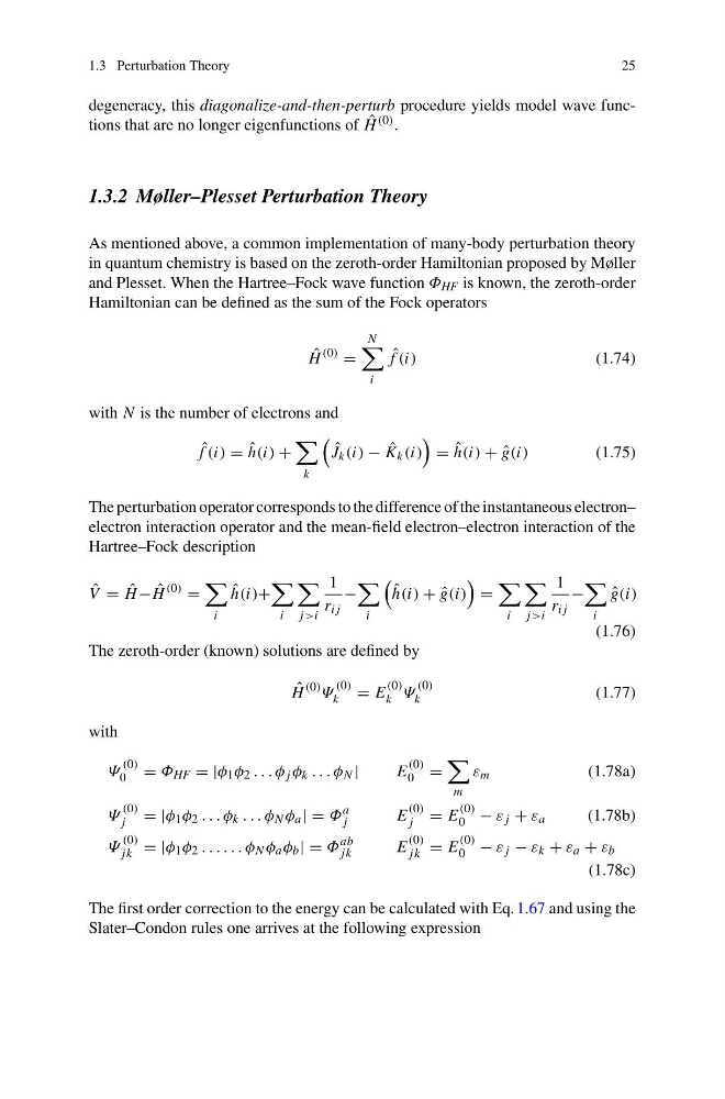
Hamiltonian can be defined as the sum of the Fock operators
ˆ
H
(0) =
N
i
ˆ
f (i)
(1.74)
with N is the number of electrons and
ˆ
f (i) = ˆ
h(i) +
k
ˆ
J k (i) − ˆ
K k (i)
= ˆ
h(i) +ˆ g(i)
(1.75)
The perturbation operator corresponds to the difference of the instantaneous electron–
electron interaction operator and the mean-field electron–electron interaction of the
Hartree–Fock description
ˆ
V = ˆ
H − ˆ
H
(0) =
i
ˆ
h(i)+
i
j>i
1
r ij
−
i
ˆ
h(i) +ˆ g(i)
=
i
j>i
1
r ij
−
i
ˆ
g(i)
(1.76)
The zeroth-order (known) solutions are defined by
ˆ
H
(0) Ψ
(0)
k = E
(0)
k Ψ
(0)
k
(1.77)
with
Ψ
(0)
0 = Φ HF =|φ 1 φ 2 ...φ j φ k ...φ N |
E
(0)
0 =
m
ε m
(1.78a)
Ψ
(0)
j =|φ 1 φ 2 ...φ k ...φ N φ a |=Φ
a
j
E
(0)
j = E
(0)
0 − ε j + ε a
(1.78b)
Ψ
(0)
jk =|φ 1 φ 2 ......φ N φ a φ b |=Φ
ab
jk
E
(0)
jk = E
(0)
0 − ε j − ε k + ε a + ε b
(1.78c)
The first order correction to the energy can be calculated with Eq. 1.67 and using the
Slater–Condon rules one arrives at the following expression
25
degeneracy, this diagonalize-and-then-perturb procedure yields model wave functions that are no longer eigenfunctions of ˆ
H (0) .
1.3.2 Møller–Plesset Perturbation Theory
As mentioned above, a common implementation of many-body perturbation theory
in quantum chemistry is based on the zeroth-order Hamiltonian proposed by Møller
and Plesset. When the Hartree–Fock wave function Φ HF is known, the zeroth-order
Hamiltonian can be defined as the sum of the Fock operators
ˆ
H
(0) =
N
i
ˆ
f (i)
(1.74)
with N is the number of electrons and
ˆ
f (i) = ˆ
h(i) +
k
ˆ
J k (i) − ˆ
K k (i)
= ˆ
h(i) +ˆ g(i)
(1.75)
The perturbation operator corresponds to the difference of the instantaneous electron–
electron interaction operator and the mean-field electron–electron interaction of the
Hartree–Fock description
ˆ
V = ˆ
H − ˆ
H
(0) =
i
ˆ
h(i)+
i
j>i
1
r ij
−
i
ˆ
h(i) +ˆ g(i)
=
i
j>i
1
r ij
−
i
ˆ
g(i)
(1.76)
The zeroth-order (known) solutions are defined by
ˆ
H
(0) Ψ
(0)
k = E
(0)
k Ψ
(0)
k
(1.77)
with
Ψ
(0)
0 = Φ HF =|φ 1 φ 2 ...φ j φ k ...φ N |
E
(0)
0 =
m
ε m
(1.78a)
Ψ
(0)
j =|φ 1 φ 2 ...φ k ...φ N φ a |=Φ
a
j
E
(0)
j = E
(0)
0 − ε j + ε a
(1.78b)
Ψ
(0)
jk =|φ 1 φ 2 ......φ N φ a φ b |=Φ
ab
jk
E
(0)
jk = E
(0)
0 − ε j − ε k + ε a + ε b
(1.78c)
The first order correction to the energy can be calculated with Eq. 1.67 and using the
Slater–Condon rules one arrives at the following expression