

1.3 Perturbation Theory
23
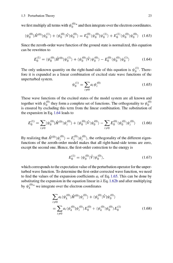
we first multiply all terms with ψ
(0)
0
∗ and then integrate over the electron coordinates.
ψ
(0)
0 | ˆ
H
(0) |ψ
(1)
0 ++ψ
(0)
0 | ˆ
V |ψ
(0)
0 =E
(0)
0 ψ
(0)
0 |ψ
(1)
0 +E
(1)
0 ψ
(0)
0 |ψ
(0)
0 (1.63)
Since the zeroth-order wave function of the ground state is normalized, this equation
can be rewritten to
E
(1)
0 ==ψ
(0)
0 | ˆ
H
(0) |ψ
(1)
0 ++ψ
(0)
0 | ˆ
V |ψ
(0)
0 −E
(0)
0 ψ
(0)
0 |ψ
(1)
0
(1.64)
The only unknown quantity on the right-hand-side of this equation is ψ
(1)
0 . Therefore it is expanded as a linear combination of excited state wave functions of the
unperturbed system.
ψ
(1)
0 =
i =0
a i ψ
(0)
i
(1.65)
These wave functions of the excited states of the model system are all known and
together with ψ
(0)
0 they form a complete set of functions. The orthogonality to ψ
(0)
0
is ensured by excluding this term from the linear combination. The substitution of
the expansion in Eq. 1.64 leads to
E
(1)
0 =
i =0
ψ
(0)
0 | ˆ
H
(0) |ψ
(0)
i ++ψ
(0)
0 | ˆ
V |ψ
(0)
0 −
i =0
E
(0)
0 ψ
(0)
0 |ψ
(0)
i
(1.66)
By realizing that ˆ
H (0) |ψ
(0)
i =E
(0)
i |ψ
(0)
i , the orthogonality of the different eigenfunctions of the zeroth-order model makes that all right-hand-side terms are zero,
except the second one. Hence, the first-order correction to the energy is
E
(1)
0 ==ψ
(0)
0 | ˆ
V |ψ
(0)
0 ,
(1.67)
which corresponds to the expectation value of the perturbation operator for the unperturbed wave function. To determine the first-order corrected wave function, we need
to find the values of the expansion coefficients a i of Eq. 1.65. This can be done by
substituting the expansion in the equation linear in λ Eq. 1.62b and after multiplying
by ψ
(0)
k
∗ we integrate over the electron coordinates
i =0
a i ψ
(0)
k | ˆ
H
(0) |ψ
(0)
i ++ψ
(0)
k | ˆ
V |ψ
(0)
0
=
i =0
a i ψ
(0)
k |ψ
(0)
i E
(0)
0 ++ψ
(0)
k |ψ
(0)
0 E
(1)
0
(1.68)
23
we first multiply all terms with ψ
(0)
0
∗ and then integrate over the electron coordinates.
ψ
(0)
0 | ˆ
H
(0) |ψ
(1)
0 ++ψ
(0)
0 | ˆ
V |ψ
(0)
0 =E
(0)
0 ψ
(0)
0 |ψ
(1)
0 +E
(1)
0 ψ
(0)
0 |ψ
(0)
0 (1.63)
Since the zeroth-order wave function of the ground state is normalized, this equation
can be rewritten to
E
(1)
0 ==ψ
(0)
0 | ˆ
H
(0) |ψ
(1)
0 ++ψ
(0)
0 | ˆ
V |ψ
(0)
0 −E
(0)
0 ψ
(0)
0 |ψ
(1)
0
(1.64)
The only unknown quantity on the right-hand-side of this equation is ψ
(1)
0 . Therefore it is expanded as a linear combination of excited state wave functions of the
unperturbed system.
ψ
(1)
0 =
i =0
a i ψ
(0)
i
(1.65)
These wave functions of the excited states of the model system are all known and
together with ψ
(0)
0 they form a complete set of functions. The orthogonality to ψ
(0)
0
is ensured by excluding this term from the linear combination. The substitution of
the expansion in Eq. 1.64 leads to
E
(1)
0 =
i =0
ψ
(0)
0 | ˆ
H
(0) |ψ
(0)
i ++ψ
(0)
0 | ˆ
V |ψ
(0)
0 −
i =0
E
(0)
0 ψ
(0)
0 |ψ
(0)
i
(1.66)
By realizing that ˆ
H (0) |ψ
(0)
i =E
(0)
i |ψ
(0)
i , the orthogonality of the different eigenfunctions of the zeroth-order model makes that all right-hand-side terms are zero,
except the second one. Hence, the first-order correction to the energy is
E
(1)
0 ==ψ
(0)
0 | ˆ
V |ψ
(0)
0 ,
(1.67)
which corresponds to the expectation value of the perturbation operator for the unperturbed wave function. To determine the first-order corrected wave function, we need
to find the values of the expansion coefficients a i of Eq. 1.65. This can be done by
substituting the expansion in the equation linear in λ Eq. 1.62b and after multiplying
by ψ
(0)
k
∗ we integrate over the electron coordinates
i =0
a i ψ
(0)
k | ˆ
H
(0) |ψ
(0)
i ++ψ
(0)
k | ˆ
V |ψ
(0)
0
=
i =0
a i ψ
(0)
k |ψ
(0)
i E
(0)
0 ++ψ
(0)
k |ψ
(0)
0 E
(1)
0
(1.68)