

1.2 Generation of Many Electron Spin Functions
19
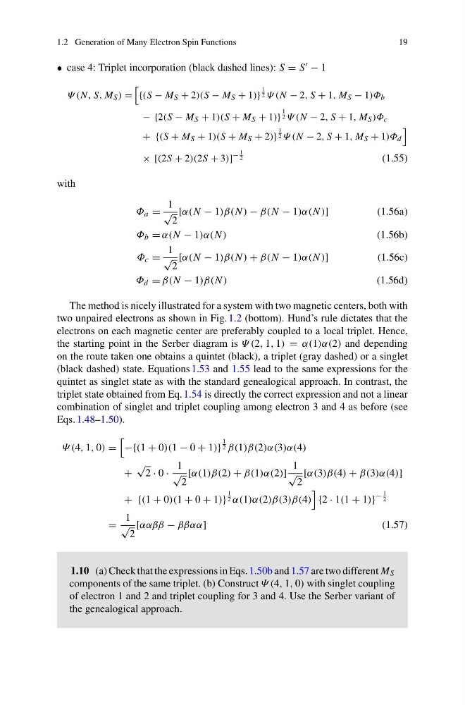
• case 4: Triplet incorporation (black dashed lines): S = S ′ − 1
Ψ(N , S, M S ) =
{(S − M S + 2)(S − M S + 1)}
1
2 Ψ(N − 2, S + 1, M S − 1)Φ b
−{ 2(S − M S + 1)(S + M S + 1)}
1
2 Ψ(N − 2, S + 1, M S )Φ c
+{ (S + M S + 1)(S + M S + 2)}
1
2 Ψ(N − 2, S + 1, M S + 1)Φ d
×[ (2S + 2)(2S + 3)]
−
1
2
(1.55)
with
Φ a =
1
√
2
[α(N − 1)β(N ) − β(N − 1)α(N )]
(1.56a)
Φ b = α(N − 1)α(N )
(1.56b)
Φ c =
1
√
2
[α(N − 1)β(N ) + β(N − 1)α(N )]
(1.56c)
Φ d = β(N − 1)β(N )
(1.56d)
The method is nicely illustrated for a system with two magnetic centers, both with
two unpaired electrons as shown in Fig. 1.2 (bottom). Hund’s rule dictates that the
electrons on each magnetic center are preferably coupled to a local triplet. Hence,
the starting point in the Serber diagram is Ψ(2, 1, 1) = α(1)α(2) and depending
on the route taken one obtains a quintet (black), a triplet (gray dashed) or a singlet
(black dashed) state. Equations 1.53 and 1.55 lead to the same expressions for the
quintet as singlet state as with the standard genealogical approach. In contrast, the
triplet state obtained from Eq. 1.54 is directly the correct expression and not a linear
combination of singlet and triplet coupling among electron 3 and 4 as before (see
Eqs. 1.48–1.50).
Ψ(4, 1, 0) =
−{(1 + 0)(1 − 0 + 1)}
1
2 β(1)β(2)α(3)α(4)
+
√
2 · 0 ·
1
√
2
[α(1)β(2) + β(1)α(2)]
1
√
2
[α(3)β(4) + β(3)α(4)]
+{ (1 + 0)(1 + 0 + 1)}
1
2 α(1)α(2)β(3)β(4)
{2 · 1(1 + 1)}
−
1
2
=
1
√
2
[ααββ − ββαα]
(1.57)
1.10 (a) Check that the expressions in Eqs. 1.50b and 1.57 are two different M S
components of the same triplet. (b) Construct Ψ(4, 1, 0) with singlet coupling
of electron 1 and 2 and triplet coupling for 3 and 4. Use the Serber variant of
the genealogical approach.
19
• case 4: Triplet incorporation (black dashed lines): S = S ′ − 1
Ψ(N , S, M S ) =
{(S − M S + 2)(S − M S + 1)}
1
2 Ψ(N − 2, S + 1, M S − 1)Φ b
−{ 2(S − M S + 1)(S + M S + 1)}
1
2 Ψ(N − 2, S + 1, M S )Φ c
+{ (S + M S + 1)(S + M S + 2)}
1
2 Ψ(N − 2, S + 1, M S + 1)Φ d
×[ (2S + 2)(2S + 3)]
−
1
2
(1.55)
with
Φ a =
1
√
2
[α(N − 1)β(N ) − β(N − 1)α(N )]
(1.56a)
Φ b = α(N − 1)α(N )
(1.56b)
Φ c =
1
√
2
[α(N − 1)β(N ) + β(N − 1)α(N )]
(1.56c)
Φ d = β(N − 1)β(N )
(1.56d)
The method is nicely illustrated for a system with two magnetic centers, both with
two unpaired electrons as shown in Fig. 1.2 (bottom). Hund’s rule dictates that the
electrons on each magnetic center are preferably coupled to a local triplet. Hence,
the starting point in the Serber diagram is Ψ(2, 1, 1) = α(1)α(2) and depending
on the route taken one obtains a quintet (black), a triplet (gray dashed) or a singlet
(black dashed) state. Equations 1.53 and 1.55 lead to the same expressions for the
quintet as singlet state as with the standard genealogical approach. In contrast, the
triplet state obtained from Eq. 1.54 is directly the correct expression and not a linear
combination of singlet and triplet coupling among electron 3 and 4 as before (see
Eqs. 1.48–1.50).
Ψ(4, 1, 0) =
−{(1 + 0)(1 − 0 + 1)}
1
2 β(1)β(2)α(3)α(4)
+
√
2 · 0 ·
1
√
2
[α(1)β(2) + β(1)α(2)]
1
√
2
[α(3)β(4) + β(3)α(4)]
+{ (1 + 0)(1 + 0 + 1)}
1
2 α(1)α(2)β(3)β(4)
{2 · 1(1 + 1)}
−
1
2
=
1
√
2
[ααββ − ββαα]
(1.57)
1.10 (a) Check that the expressions in Eqs. 1.50b and 1.57 are two different M S
components of the same triplet. (b) Construct Ψ(4, 1, 0) with singlet coupling
of electron 1 and 2 and triplet coupling for 3 and 4. Use the Serber variant of
the genealogical approach.