

130
4 From Orbital Models to Accurate Predictions
and C is an appropriate constant shift to ensure that ˆ
H
(0)
D is equivalent to the full
Hamiltonian in the active part.
Contracted versus uncontracted: The simplest way to define the first-order wave
function is to apply single and double excitation operators on all the determinants
(or CSFs) of the reference wave function.
ψ
(1) =
I
rstu
c I,rstu ˆ
E rs ˆ
E tu Φ I
(4.49)
The second-order correction to the energy is relatively straightforward to evaluate,
but the number of terms in the summation rapidly becomes very large, especially for
large reference wave functions. A second approach is to apply excitation operators
not on the individual determinants of CSFs of the reference space, but on the reference
wave function as a whole.
ψ
(1) =
rstu
c rstu ˆ
E rs ˆ
E tu ψ
(0)
(4.50)
This approach generates much less terms since the external determinants appear
as contracted sums in the first-order wave function. Moreover, the dimension of the
external space does not grow as fast with the size of ψ (1) as in the uncontracted way of
generating ψ (1) . On the other hand, the calculation of the second-order correction to
the energy relies on significantly more complicated expressions but once programmed
this is just a minor issue compared to the limited length of ψ (1) .
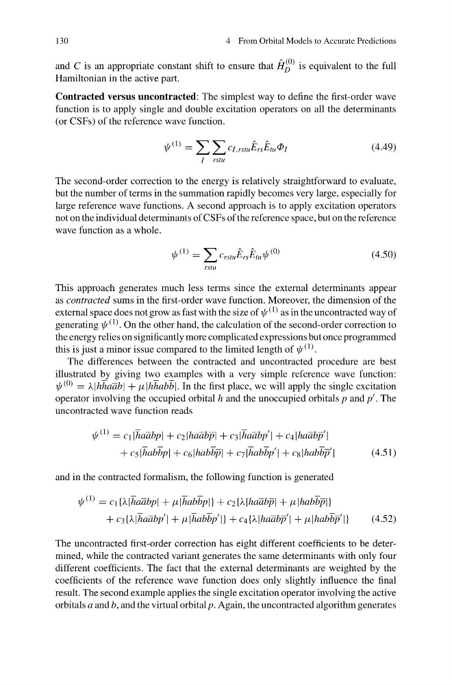
The differences between the contracted and uncontracted procedure are best
illustrated by giving two examples with a very simple reference wave function:
ψ (0) = λ|hhaab|+µ|hhabb|. In the first place, we will apply the single excitation
operator involving the occupied orbital h and the unoccupied orbitals p and p ′ .The
uncontracted wave function reads
ψ
(1) = c 1 |haabp|+c 2 |haabp|+c 3 |haabp
′ |+c 4 |haabp
′ |
+ c 5 |habbp|+c 6 |habbp|+c 7 |habbp
′ |+c 8 |habbp
′ |
(4.51)
and in the contracted formalism, the following function is generated
ψ
(1) = c 1 {λ|haabp|+µ|habbp|} + c 2 {λ|haabp|+µ|habbp|}
+ c 3 {λ|haabp
′ |+µ|habbp
′ |} + c 4 {λ|haabp
′ |+µ|habbp
′ |}
(4.52)
The uncontracted first-order correction has eight different coefficients to be determined, while the contracted variant generates the same determinants with only four
different coefficients. The fact that the external determinants are weighted by the
coefficients of the reference wave function does only slightly influence the final
result. The second example applies the single excitation operator involving the active
orbitals a and b, and the virtual orbital p. Again, the uncontracted algorithm generates
4 From Orbital Models to Accurate Predictions
and C is an appropriate constant shift to ensure that ˆ
H
(0)
D is equivalent to the full
Hamiltonian in the active part.
Contracted versus uncontracted: The simplest way to define the first-order wave
function is to apply single and double excitation operators on all the determinants
(or CSFs) of the reference wave function.
ψ
(1) =
I
rstu
c I,rstu ˆ
E rs ˆ
E tu Φ I
(4.49)
The second-order correction to the energy is relatively straightforward to evaluate,
but the number of terms in the summation rapidly becomes very large, especially for
large reference wave functions. A second approach is to apply excitation operators
not on the individual determinants of CSFs of the reference space, but on the reference
wave function as a whole.
ψ
(1) =
rstu
c rstu ˆ
E rs ˆ
E tu ψ
(0)
(4.50)
This approach generates much less terms since the external determinants appear
as contracted sums in the first-order wave function. Moreover, the dimension of the
external space does not grow as fast with the size of ψ (1) as in the uncontracted way of
generating ψ (1) . On the other hand, the calculation of the second-order correction to
the energy relies on significantly more complicated expressions but once programmed
this is just a minor issue compared to the limited length of ψ (1) .
The differences between the contracted and uncontracted procedure are best
illustrated by giving two examples with a very simple reference wave function:
ψ (0) = λ|hhaab|+µ|hhabb|. In the first place, we will apply the single excitation
operator involving the occupied orbital h and the unoccupied orbitals p and p ′ .The
uncontracted wave function reads
ψ
(1) = c 1 |haabp|+c 2 |haabp|+c 3 |haabp
′ |+c 4 |haabp
′ |
+ c 5 |habbp|+c 6 |habbp|+c 7 |habbp
′ |+c 8 |habbp
′ |
(4.51)
and in the contracted formalism, the following function is generated
ψ
(1) = c 1 {λ|haabp|+µ|habbp|} + c 2 {λ|haabp|+µ|habbp|}
+ c 3 {λ|haabp
′ |+µ|habbp
′ |} + c 4 {λ|haabp
′ |+µ|habbp
′ |}
(4.52)
The uncontracted first-order correction has eight different coefficients to be determined, while the contracted variant generates the same determinants with only four
different coefficients. The fact that the external determinants are weighted by the
coefficients of the reference wave function does only slightly influence the final
result. The second example applies the single excitation operator involving the active
orbitals a and b, and the virtual orbital p. Again, the uncontracted algorithm generates