

122
4 From Orbital Models to Accurate Predictions
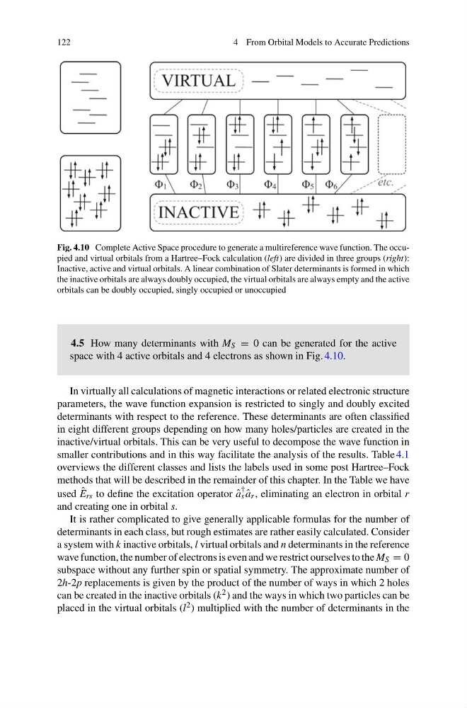
Fig. 4.10 Complete Active Space procedure to generate a multireference wave function. The occupied and virtual orbitals from a Hartree–Fock calculation (left) are divided in three groups (right):
Inactive, active and virtual orbitals. A linear combination of Slater determinants is formed in which
the inactive orbitals are always doubly occupied, the virtual orbitals are always empty and the active
orbitals can be doubly occupied, singly occupied or unoccupied
4.5 How many determinants with M S = 0 can be generated for the active
space with 4 active orbitals and 4 electrons as shown in Fig. 4.10.
In virtually all calculations of magnetic interactions or related electronic structure
parameters, the wave function expansion is restricted to singly and doubly excited
determinants with respect to the reference. These determinants are often classified
in eight different groups depending on how many holes/particles are created in the
inactive/virtual orbitals. This can be very useful to decompose the wave function in
smaller contributions and in this way facilitate the analysis of the results. Table 4.1
overviews the different classes and lists the labels used in some post Hartree–Fock
methods that will be described in the remainder of this chapter. In the Table we have
used ˆ
E rs to define the excitation operator ˆ
a
†
s ˆ
a r , eliminating an electron in orbital r
and creating one in orbital s.
It is rather complicated to give generally applicable formulas for the number of
determinants in each class, but rough estimates are rather easily calculated. Consider
a system with k inactive orbitals, l virtual orbitals and n determinants in the reference
wave function, the number of electrons is even and we restrict ourselves to the M S = 0
subspace without any further spin or spatial symmetry. The approximate number of
2h-2p replacements is given by the product of the number of ways in which 2 holes
can be created in the inactive orbitals (k 2 ) and the ways in which two particles can be
placed in the virtual orbitals (l 2 ) multiplied with the number of determinants in the
4 From Orbital Models to Accurate Predictions
Fig. 4.10 Complete Active Space procedure to generate a multireference wave function. The occupied and virtual orbitals from a Hartree–Fock calculation (left) are divided in three groups (right):
Inactive, active and virtual orbitals. A linear combination of Slater determinants is formed in which
the inactive orbitals are always doubly occupied, the virtual orbitals are always empty and the active
orbitals can be doubly occupied, singly occupied or unoccupied
4.5 How many determinants with M S = 0 can be generated for the active
space with 4 active orbitals and 4 electrons as shown in Fig. 4.10.
In virtually all calculations of magnetic interactions or related electronic structure
parameters, the wave function expansion is restricted to singly and doubly excited
determinants with respect to the reference. These determinants are often classified
in eight different groups depending on how many holes/particles are created in the
inactive/virtual orbitals. This can be very useful to decompose the wave function in
smaller contributions and in this way facilitate the analysis of the results. Table 4.1
overviews the different classes and lists the labels used in some post Hartree–Fock
methods that will be described in the remainder of this chapter. In the Table we have
used ˆ
E rs to define the excitation operator ˆ
a
†
s ˆ
a r , eliminating an electron in orbital r
and creating one in orbital s.
It is rather complicated to give generally applicable formulas for the number of
determinants in each class, but rough estimates are rather easily calculated. Consider
a system with k inactive orbitals, l virtual orbitals and n determinants in the reference
wave function, the number of electrons is even and we restrict ourselves to the M S = 0
subspace without any further spin or spatial symmetry. The approximate number of
2h-2p replacements is given by the product of the number of ways in which 2 holes
can be created in the inactive orbitals (k 2 ) and the ways in which two particles can be
placed in the virtual orbitals (l 2 ) multiplied with the number of determinants in the