

3.4 Complex Interactions
89
3.9 Calculate the outcome of (ˆ s + (1) +ˆ s + (2))(ˆ s − (3) +ˆ s − (4)), (ˆ s − (1) +
ˆ
s − (2))(ˆ s + (3) +ˆ s + (4)) and (ˆ s z (1) +ˆ s z (2))(ˆ s z (3) +ˆ s z (4)) acting on ααββ,
ββαα, αβαβ, αββα, βαβα and βααβ. Use the results to verify the Heisenberg
Hamiltonian eigenvalues of the singlet and triplet spin functions.
As long as magnetic anisotropy can be neglected, the regular spacing between
the energy levels, the Landé pattern of Eq. 3.29 gives a very accurate representation
of the experimental situation. However, sometimes deviations have been observed,
which are usually ascribed to biquadratic interactions and subsequently incorporated
in the model by adding an extra term to the Heisenberg Hamiltonian
ˆ
H =−J ˆ
S 1 · ˆ
S 2 + λ( ˆ
S 1 · ˆ
S 2 )
2
(3.72)
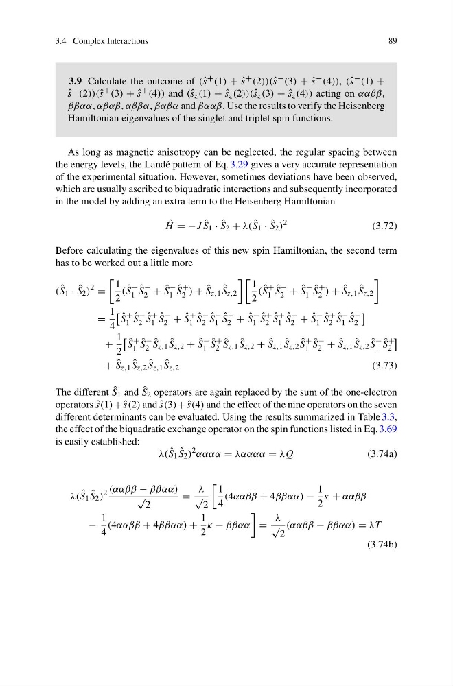
Before calculating the eigenvalues of this new spin Hamiltonian, the second term
has to be worked out a little more
( ˆ
S 1 · ˆ
S 2 )
2 =
1
2
( ˆ
S
+
1
ˆ
S
−
2 + ˆ
S
−
1
ˆ
S
+
2 ) + ˆ
S z,1 ˆ
S z,2
1
2
( ˆ
S
+
1
ˆ
S
−
2 + ˆ
S
−
1
ˆ
S
+
2 ) + ˆ
S z,1 ˆ
S z,2
=
1
4
ˆ
S
+
1
ˆ
S
−
2
ˆ
S
+
1
ˆ
S
−
2 + ˆ
S
+
1
ˆ
S
−
2
ˆ
S
−
1
ˆ
S
+
2 + ˆ
S
−
1
ˆ
S
+
2
ˆ
S
+
1
ˆ
S
−
2 + ˆ
S
−
1
ˆ
S
+
2
ˆ
S
−
1
ˆ
S
+
2
+
1
2
ˆ
S
+
1
ˆ
S
−
2
ˆ
S z,1 ˆ
S z,2 + ˆ
S
−
1
ˆ
S
+
2
ˆ
S z,1 ˆ
S z,2 + ˆ
S z,1 ˆ
S z,2 ˆ
S
+
1
ˆ
S
−
2 + ˆ
S z,1 ˆ
S z,2 ˆ
S
−
1
ˆ
S
+
2
+ ˆ
S z,1 ˆ
S z,2 ˆ
S z,1 ˆ
S z,2
(3.73)
The different ˆ
S 1 and ˆ
S 2 operators are again replaced by the sum of the one-electron
operators ˆ
s(1) +ˆ s(2) and ˆ
s(3) +ˆ s(4) and the effect of the nine operators on the seven
different determinants can be evaluated. Using the results summarized in Table 3.3,
the effect of the biquadratic exchange operator on the spin functions listed in Eq. 3.69
is easily established:
λ( ˆ
S 1 ˆ
S 2 )
2 αααα = λαααα = λQ
(3.74a)
λ( ˆ
S 1 ˆ
S 2 )
2 (ααββ − ββαα)
√
2
=
λ
√
2
1
4
(4ααββ + 4ββαα) −
1
2
κ + ααββ
−
1
4
(4ααββ + 4ββαα) +
1
2
κ − ββαα
=
λ
√
2
(ααββ − ββαα) = λT
(3.74b)
89
3.9 Calculate the outcome of (ˆ s + (1) +ˆ s + (2))(ˆ s − (3) +ˆ s − (4)), (ˆ s − (1) +
ˆ
s − (2))(ˆ s + (3) +ˆ s + (4)) and (ˆ s z (1) +ˆ s z (2))(ˆ s z (3) +ˆ s z (4)) acting on ααββ,
ββαα, αβαβ, αββα, βαβα and βααβ. Use the results to verify the Heisenberg
Hamiltonian eigenvalues of the singlet and triplet spin functions.
As long as magnetic anisotropy can be neglected, the regular spacing between
the energy levels, the Landé pattern of Eq. 3.29 gives a very accurate representation
of the experimental situation. However, sometimes deviations have been observed,
which are usually ascribed to biquadratic interactions and subsequently incorporated
in the model by adding an extra term to the Heisenberg Hamiltonian
ˆ
H =−J ˆ
S 1 · ˆ
S 2 + λ( ˆ
S 1 · ˆ
S 2 )
2
(3.72)
Before calculating the eigenvalues of this new spin Hamiltonian, the second term
has to be worked out a little more
( ˆ
S 1 · ˆ
S 2 )
2 =
1
2
( ˆ
S
+
1
ˆ
S
−
2 + ˆ
S
−
1
ˆ
S
+
2 ) + ˆ
S z,1 ˆ
S z,2
1
2
( ˆ
S
+
1
ˆ
S
−
2 + ˆ
S
−
1
ˆ
S
+
2 ) + ˆ
S z,1 ˆ
S z,2
=
1
4
ˆ
S
+
1
ˆ
S
−
2
ˆ
S
+
1
ˆ
S
−
2 + ˆ
S
+
1
ˆ
S
−
2
ˆ
S
−
1
ˆ
S
+
2 + ˆ
S
−
1
ˆ
S
+
2
ˆ
S
+
1
ˆ
S
−
2 + ˆ
S
−
1
ˆ
S
+
2
ˆ
S
−
1
ˆ
S
+
2
+
1
2
ˆ
S
+
1
ˆ
S
−
2
ˆ
S z,1 ˆ
S z,2 + ˆ
S
−
1
ˆ
S
+
2
ˆ
S z,1 ˆ
S z,2 + ˆ
S z,1 ˆ
S z,2 ˆ
S
+
1
ˆ
S
−
2 + ˆ
S z,1 ˆ
S z,2 ˆ
S
−
1
ˆ
S
+
2
+ ˆ
S z,1 ˆ
S z,2 ˆ
S z,1 ˆ
S z,2
(3.73)
The different ˆ
S 1 and ˆ
S 2 operators are again replaced by the sum of the one-electron
operators ˆ
s(1) +ˆ s(2) and ˆ
s(3) +ˆ s(4) and the effect of the nine operators on the seven
different determinants can be evaluated. Using the results summarized in Table 3.3,
the effect of the biquadratic exchange operator on the spin functions listed in Eq. 3.69
is easily established:
λ( ˆ
S 1 ˆ
S 2 )
2 αααα = λαααα = λQ
(3.74a)
λ( ˆ
S 1 ˆ
S 2 )
2 (ααββ − ββαα)
√
2
=
λ
√
2
1
4
(4ααββ + 4ββαα) −
1
2
κ + ααββ
−
1
4
(4ααββ + 4ββαα) +
1
2
κ − ββαα
=
λ
√
2
(ααββ − ββαα) = λT
(3.74b)