

60
Z. Amini et al.
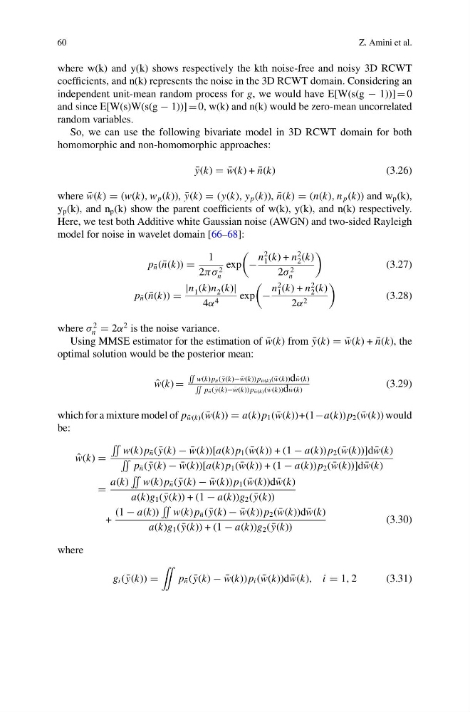
where w(k) and y(k) shows respectively the kth noise-free and noisy 3D RCWT
coefficients, and n(k) represents the noise in the 3D RCWT domain. Considering an
independent unit-mean random process for g, we would have E[W(s(g − 1))] 0
and since E[W(s)W(s(g − 1))] 0, w(k) and n(k) would be zero-mean uncorrelated
random variables.
So, we can use the following bivariate model in 3D RCWT domain for both
homomorphic and non-homomorphic approaches:
¯
y(k) ¯
w(k) + ¯
n(k)
(3.26)
where ¯
w(k) (w(k), w p (k)), ¯
y(k) (y(k), y p (k)), ¯
n(k) (n(k), n p (k)) and w p (k),
y p (k), and n p (k) show the parent coefficients of w(k), y(k), and n(k) respectively.
Here, we test both Additive white Gaussian noise (AWGN) and two-sided Rayleigh
model for noise in wavelet domain [66–68]:
p ¯
n ( ¯
n(k))
1
2πσ 2
n
exp
−
n
2
1 (k) + n
2
2 (k)
2σ 2
n
(3.27)
p ¯
n ( ¯
n(k))
|n 1 (k)n 2 (k)|
4α 4
exp
−
n
2
1 (k) + n
2
2 (k)
2α 2
(3.28)
where σ
2
n 2α
2 is the noise variance.
Using MMSE estimator for the estimation of ¯
w(k) from ¯
y(k) ¯
w(k) + ¯
n(k), the
optimal solution would be the posterior mean:
ˆ
w(k)
˜
w(k) p ¯
n ( ¯
y(k)− ¯
w(k)) p ¯
w(k) ( ¯
w(k))d ¯
w(k)
˜
p ¯
n ( ¯
y(k)− ¯
w(k)) p ¯
w(k) ( ¯
w(k))d ¯
w(k)
(3.29)
which for a mixture model of p ¯
w(k) ( ¯
w(k)) a(k) p 1 ( ¯
w(k))+(1−a(k)) p 2 ( ¯
w(k)) would
be:
ˆ
w(k)
˜
w(k) p ¯
n ( ¯
y(k) − ¯
w(k))[a(k) p 1 ( ¯
w(k)) + (1 − a(k)) p 2 ( ¯
w(k))]d ¯
w(k)
˜
p ¯
n ( ¯
y(k) − ¯
w(k))[a(k) p 1 ( ¯
w(k)) + (1 − a(k)) p 2 ( ¯
w(k))]d ¯
w(k)
a(k)
˜
w(k) p ¯
n ( ¯
y(k) − ¯
w(k)) p 1 ( ¯
w(k))d ¯
w(k)
a(k)g 1 ( ¯
y(k)) + (1 − a(k))g 2 ( ¯
y(k))
+
(1 − a(k))
˜
w(k) p ¯
n ( ¯
y(k) − ¯
w(k)) p 2 ( ¯
w(k))d ¯
w(k)
a(k)g 1 ( ¯
y(k)) + (1 − a(k))g 2 ( ¯
y(k))
(3.30)
where
g i ( ¯
y(k))
¨
p ¯
n ( ¯
y(k) − ¯
w(k)) p i ( ¯
w(k))d ¯
w(k), i 1, 2
(3.31)
Z. Amini et al.
where w(k) and y(k) shows respectively the kth noise-free and noisy 3D RCWT
coefficients, and n(k) represents the noise in the 3D RCWT domain. Considering an
independent unit-mean random process for g, we would have E[W(s(g − 1))] 0
and since E[W(s)W(s(g − 1))] 0, w(k) and n(k) would be zero-mean uncorrelated
random variables.
So, we can use the following bivariate model in 3D RCWT domain for both
homomorphic and non-homomorphic approaches:
¯
y(k) ¯
w(k) + ¯
n(k)
(3.26)
where ¯
w(k) (w(k), w p (k)), ¯
y(k) (y(k), y p (k)), ¯
n(k) (n(k), n p (k)) and w p (k),
y p (k), and n p (k) show the parent coefficients of w(k), y(k), and n(k) respectively.
Here, we test both Additive white Gaussian noise (AWGN) and two-sided Rayleigh
model for noise in wavelet domain [66–68]:
p ¯
n ( ¯
n(k))
1
2πσ 2
n
exp
−
n
2
1 (k) + n
2
2 (k)
2σ 2
n
(3.27)
p ¯
n ( ¯
n(k))
|n 1 (k)n 2 (k)|
4α 4
exp
−
n
2
1 (k) + n
2
2 (k)
2α 2
(3.28)
where σ
2
n 2α
2 is the noise variance.
Using MMSE estimator for the estimation of ¯
w(k) from ¯
y(k) ¯
w(k) + ¯
n(k), the
optimal solution would be the posterior mean:
ˆ
w(k)
˜
w(k) p ¯
n ( ¯
y(k)− ¯
w(k)) p ¯
w(k) ( ¯
w(k))d ¯
w(k)
˜
p ¯
n ( ¯
y(k)− ¯
w(k)) p ¯
w(k) ( ¯
w(k))d ¯
w(k)
(3.29)
which for a mixture model of p ¯
w(k) ( ¯
w(k)) a(k) p 1 ( ¯
w(k))+(1−a(k)) p 2 ( ¯
w(k)) would
be:
ˆ
w(k)
˜
w(k) p ¯
n ( ¯
y(k) − ¯
w(k))[a(k) p 1 ( ¯
w(k)) + (1 − a(k)) p 2 ( ¯
w(k))]d ¯
w(k)
˜
p ¯
n ( ¯
y(k) − ¯
w(k))[a(k) p 1 ( ¯
w(k)) + (1 − a(k)) p 2 ( ¯
w(k))]d ¯
w(k)
a(k)
˜
w(k) p ¯
n ( ¯
y(k) − ¯
w(k)) p 1 ( ¯
w(k))d ¯
w(k)
a(k)g 1 ( ¯
y(k)) + (1 − a(k))g 2 ( ¯
y(k))
+
(1 − a(k))
˜
w(k) p ¯
n ( ¯
y(k) − ¯
w(k)) p 2 ( ¯
w(k))d ¯
w(k)
a(k)g 1 ( ¯
y(k)) + (1 − a(k))g 2 ( ¯
y(k))
(3.30)
where
g i ( ¯
y(k))
¨
p ¯
n ( ¯
y(k) − ¯
w(k)) p i ( ¯
w(k))d ¯
w(k), i 1, 2
(3.31)