

374
F. Shi et al.
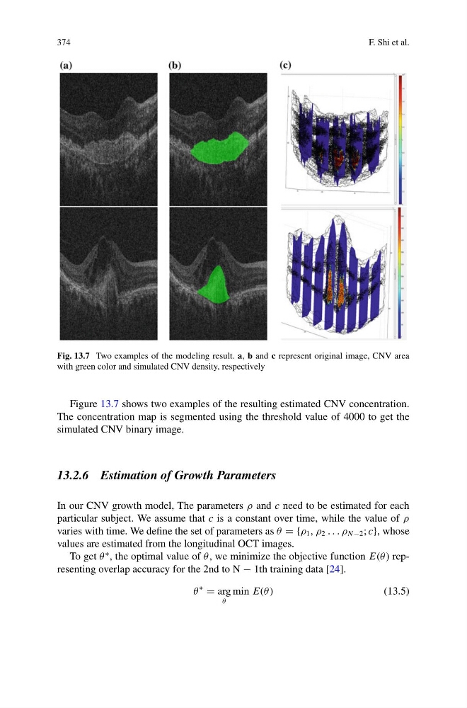
Fig. 13.7 Two examples of the modeling result. a, b and c represent original image, CNV area
with green color and simulated CNV density, respectively
Figure 13.7 shows two examples of the resulting estimated CNV concentration.
The concentration map is segmented using the threshold value of 4000 to get the
simulated CNV binary image.
13.2.6 Estimation of Growth Parameters
In our CNV growth model, The parameters ρ and c need to be estimated for each
particular subject. We assume that c is a constant over time, while the value of ρ
varies with time. We define the set of parameters as θ {ρ 1 , ρ 2 . . . ρ N −2 ; c}, whose
values are estimated from the longitudinal OCT images.
To get θ
∗ , the optimal value of θ , we minimize the objective function E(θ ) representing overlap accuracy for the 2nd to N − 1th training data [24].
θ
∗
arg
θ
min E(θ )
(13.5)
F. Shi et al.
Fig. 13.7 Two examples of the modeling result. a, b and c represent original image, CNV area
with green color and simulated CNV density, respectively
Figure 13.7 shows two examples of the resulting estimated CNV concentration.
The concentration map is segmented using the threshold value of 4000 to get the
simulated CNV binary image.
13.2.6 Estimation of Growth Parameters
In our CNV growth model, The parameters ρ and c need to be estimated for each
particular subject. We assume that c is a constant over time, while the value of ρ
varies with time. We define the set of parameters as θ {ρ 1 , ρ 2 . . . ρ N −2 ; c}, whose
values are estimated from the longitudinal OCT images.
To get θ
∗ , the optimal value of θ , we minimize the objective function E(θ ) representing overlap accuracy for the 2nd to N − 1th training data [24].
θ
∗
arg
θ
min E(θ )
(13.5)