

314
Q. Chen et al.
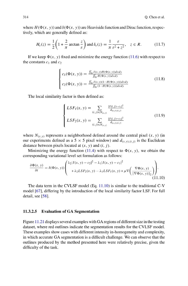
where H ((x, y)) and δ((x, y)) are Heaviside function and Dirac function, respectively, which are generally defined as:
H ε (z)
1
2
1 +
2
π
arctan
z
ε
and δ ε (z)
1
π
ε
ε 2 + z 2 , z ∈ R.
(11.7)
If we keep (x, y) fixed and minimize the energy function (11.6) with respect to
the constants c 1 and c 2
⎧
⎪ ⎪ ⎨
⎪ ⎪ ⎩
c 1 ((x, y))
˜
I (x,y)H ((x,y))dxdy
˜
H ((x,y))dxdy
c 2 ((x, y))
˜
I (x,y)(1−H ((x,y)))dxdy
˜
(1−H ((x,y)))dxdy
(11.8)
The local similarity factor is then defined as:
⎧
⎪ ⎪ ⎪ ⎨
⎪ ⎪ ⎪ ⎩
L S F 1 (x, y)
(i, j)∈N (x,y)
|I (i, j)−c 1 |
2
d (x,y),(i, j)
L S F 2 (x, y)
(i, j)∈N (x,y)
|I (i, j)−c 2 |
2
d (x,y),(i, j)
(11.9)
where N (x,y) represents a neighborhood defined around the central pixel (x, y) (in
our experiments defined as a 5 × 5 pixel window) and d (x,y),(i, j) is the Euclidean
distance between pixels located at (x, y) and (i, j).
Minimizing the energy function (11.4) with respect to (x, y), we obtain the
corresponding variational level set formulation as follows:
∂∂(x, y)
∂t
δ((x, y))
⎛
⎜
⎝
λ 2 |I (x, y) − c 2 |
2 − λ 1 |I (x, y) − c 1 |
2
+ λ 2 L SF 2 (x, y) − λ 1 L SF 1 (x, y) + μ∇
∇(x, y)
∇(x, y) 2
⎞
⎟
⎠.
(11.10)
The data term in the CVLSF model (Eq. 11.10) is similar to the traditional C-V
model [67], differing by the introduction of the local similarity factor LSF. For full
detail, see [58].
11.3.2.5 Evaluation of GA Segmentation
Figure 11.21 displays several examples with GA regions of different size in the testing
dataset, where red outlines indicate the segmentation results for the CVLSF model.
These examples show cases with different intensity in-homogeneity and complexity,
in which accurate GA segmentation is a difficult challenge. We can observe that the
outlines produced by the method presented here were relatively precise, given the
difficulty of the task.
Q. Chen et al.
where H ((x, y)) and δ((x, y)) are Heaviside function and Dirac function, respectively, which are generally defined as:
H ε (z)
1
2
1 +
2
π
arctan
z
ε
and δ ε (z)
1
π
ε
ε 2 + z 2 , z ∈ R.
(11.7)
If we keep (x, y) fixed and minimize the energy function (11.6) with respect to
the constants c 1 and c 2
⎧
⎪ ⎪ ⎨
⎪ ⎪ ⎩
c 1 ((x, y))
˜
I (x,y)H ((x,y))dxdy
˜
H ((x,y))dxdy
c 2 ((x, y))
˜
I (x,y)(1−H ((x,y)))dxdy
˜
(1−H ((x,y)))dxdy
(11.8)
The local similarity factor is then defined as:
⎧
⎪ ⎪ ⎪ ⎨
⎪ ⎪ ⎪ ⎩
L S F 1 (x, y)
(i, j)∈N (x,y)
|I (i, j)−c 1 |
2
d (x,y),(i, j)
L S F 2 (x, y)
(i, j)∈N (x,y)
|I (i, j)−c 2 |
2
d (x,y),(i, j)
(11.9)
where N (x,y) represents a neighborhood defined around the central pixel (x, y) (in
our experiments defined as a 5 × 5 pixel window) and d (x,y),(i, j) is the Euclidean
distance between pixels located at (x, y) and (i, j).
Minimizing the energy function (11.4) with respect to (x, y), we obtain the
corresponding variational level set formulation as follows:
∂∂(x, y)
∂t
δ((x, y))
⎛
⎜
⎝
λ 2 |I (x, y) − c 2 |
2 − λ 1 |I (x, y) − c 1 |
2
+ λ 2 L SF 2 (x, y) − λ 1 L SF 1 (x, y) + μ∇
∇(x, y)
∇(x, y) 2
⎞
⎟
⎠.
(11.10)
The data term in the CVLSF model (Eq. 11.10) is similar to the traditional C-V
model [67], differing by the introduction of the local similarity factor LSF. For full
detail, see [58].
11.3.2.5 Evaluation of GA Segmentation
Figure 11.21 displays several examples with GA regions of different size in the testing
dataset, where red outlines indicate the segmentation results for the CVLSF model.
These examples show cases with different intensity in-homogeneity and complexity,
in which accurate GA segmentation is a difficult challenge. We can observe that the
outlines produced by the method presented here were relatively precise, given the
difficulty of the task.