

260
F. Shi et al.
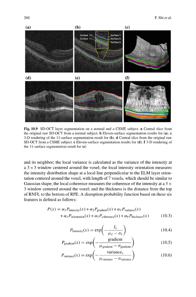
Fig. 10.9 SD-OCT layer segmentation on a normal and a CSME subject. a Central slice from
the original raw SD-OCT from a normal subject. b Eleven-surface segmentation results for (a). c
3-D rendering of the 11-surface segmentation result for (b). d Central slice from the original raw
SD-OCT from a CSME subject. e Eleven-surface segmentation results for (d). f 3-D rendering of
the 11-surface segmentation result for (e)
and its neighbor; the local variance is calculated as the variance of the intensity at
a 3 × 3 window centered around the voxel; the local intensity orientation measures
the intensity distribution shape at a local line perpendicular to the ELM layer orientation centered around the voxel, with length of 7 voxels, which should be similar to
Gaussian shape; the local coherence measures the coherence of the intensity at a 3 ×
3 window centered around the voxel; and the thickness is the distance from the top
of RNFL to the bottom of RPE. A disruption probability function based on these six
features is defined as follows:
P(x) α 1 P intensity (x) + α 2 P gradient (x) + α 3 P variance (x)
+ α 4 P orientation (x) + α 5 P coherence (x) + α 6 P thickness (x)
(10.3)
P intensity (x) exp
−
I x
μ I − σ I
(10.4)
P gradient (x) exp
−
gradient
μ gradient − σ gradient
(10.5)
P variance (x) exp
−
variance x
μ variance − σ variance
(10.6)
F. Shi et al.
Fig. 10.9 SD-OCT layer segmentation on a normal and a CSME subject. a Central slice from
the original raw SD-OCT from a normal subject. b Eleven-surface segmentation results for (a). c
3-D rendering of the 11-surface segmentation result for (b). d Central slice from the original raw
SD-OCT from a CSME subject. e Eleven-surface segmentation results for (d). f 3-D rendering of
the 11-surface segmentation result for (e)
and its neighbor; the local variance is calculated as the variance of the intensity at
a 3 × 3 window centered around the voxel; the local intensity orientation measures
the intensity distribution shape at a local line perpendicular to the ELM layer orientation centered around the voxel, with length of 7 voxels, which should be similar to
Gaussian shape; the local coherence measures the coherence of the intensity at a 3 ×
3 window centered around the voxel; and the thickness is the distance from the top
of RNFL to the bottom of RPE. A disruption probability function based on these six
features is defined as follows:
P(x) α 1 P intensity (x) + α 2 P gradient (x) + α 3 P variance (x)
+ α 4 P orientation (x) + α 5 P coherence (x) + α 6 P thickness (x)
(10.3)
P intensity (x) exp
−
I x
μ I − σ I
(10.4)
P gradient (x) exp
−
gradient
μ gradient − σ gradient
(10.5)
P variance (x) exp
−
variance x
μ variance − σ variance
(10.6)