

218
K. K. Vupparaboina et al.
B. Refinement via eigenvalue analysis of the Hessian matrix: To remove such discontinuities, an adaptive Hessian analysis method is adopted [32, 33]. In particular, first whether a pixel belongs to a blood vessel (present only in the choroid)
or not is found. To this end, we estimate the Hessian matrix H at every pixel
based on its neighborhood, compute the eigenvalues λ 1 and λ 2 of H, and verify whether λ 1 is small and λ 2 is large, which has been shown to correspond
to dark tubular structures such as choroidal blood vessels [34]. To complicate
matters, the intensities across the length of the scan was not uniform, and hence
a unique threshold pair on the eigenvalues may not suffice in detecting choroid
vessel cross-sections accurately. Accordingly, to improve accuracy, thresholds
on λ 1 and λ 2 are picked in an adaptive manner, and add the outer boundary of
newly detected choroid vessels to our initial COB estimate, thereby removing
undesirable discontinuities (Fig. 9.4k).
C. Smooth interpolation using tensor voting: The refined COB estimate appears to
divide the choroidal granularity and the scleral uniformity adequately, albeit in
jagged manner. In contrast, manual delineation of the COB by an expert is generally smooth (Fig. 9.4l). To achieve similar smoothness in our automated COB
estimate, tensor voting is adopted [35, 36]. Directly applying tensor voting on
the refined COB estimate may lead to omission of some choroid vessels, because
final boundary may pass through the choroid layer cutting some of the blood vessels. Therefore, post preprocessing is performed on the refined COB estimate,
which involves discarding boundary pixels that are close to local minima. This
is done by dividing each scan into three windows along the length and fixing
a local threshold based on mean thickness value of the corresponding window.
Further, threshold is chosen slightly greater than the local mean. Before proceeding further, we describe in brief the tensor voting technique, which propagates
information using tokens, conveying various objects’ orientation preferences
(i.e., votes) to their neighbors. When such votes are tallied, objects belonging to
the same structure tend to join together. The influence of a vote decays away from
the object, and the saliency decay function (DF) is generally taken as Gaussian:
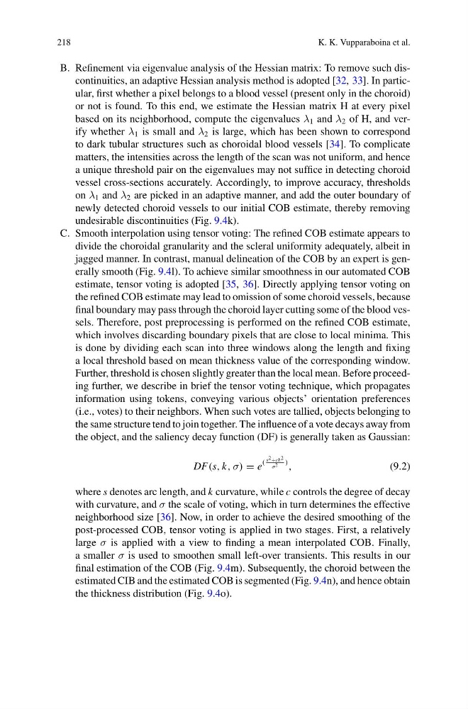
DF(s, k, σ) = e
(
s 2 +ck 2
σ 2 ) ,
(9.2)
where s denotes arc length, and k curvature, while c controls the degree of decay
with curvature, and σ the scale of voting, which in turn determines the effective
neighborhood size [36]. Now, in order to achieve the desired smoothing of the
post-processed COB, tensor voting is applied in two stages. First, a relatively
large σ is applied with a view to finding a mean interpolated COB. Finally,
a smaller σ is used to smoothen small left-over transients. This results in our
final estimation of the COB (Fig. 9.4m). Subsequently, the choroid between the
estimated CIB and the estimated COB is segmented (Fig. 9.4n), and hence obtain
the thickness distribution (Fig. 9.4o).
K. K. Vupparaboina et al.
B. Refinement via eigenvalue analysis of the Hessian matrix: To remove such discontinuities, an adaptive Hessian analysis method is adopted [32, 33]. In particular, first whether a pixel belongs to a blood vessel (present only in the choroid)
or not is found. To this end, we estimate the Hessian matrix H at every pixel
based on its neighborhood, compute the eigenvalues λ 1 and λ 2 of H, and verify whether λ 1 is small and λ 2 is large, which has been shown to correspond
to dark tubular structures such as choroidal blood vessels [34]. To complicate
matters, the intensities across the length of the scan was not uniform, and hence
a unique threshold pair on the eigenvalues may not suffice in detecting choroid
vessel cross-sections accurately. Accordingly, to improve accuracy, thresholds
on λ 1 and λ 2 are picked in an adaptive manner, and add the outer boundary of
newly detected choroid vessels to our initial COB estimate, thereby removing
undesirable discontinuities (Fig. 9.4k).
C. Smooth interpolation using tensor voting: The refined COB estimate appears to
divide the choroidal granularity and the scleral uniformity adequately, albeit in
jagged manner. In contrast, manual delineation of the COB by an expert is generally smooth (Fig. 9.4l). To achieve similar smoothness in our automated COB
estimate, tensor voting is adopted [35, 36]. Directly applying tensor voting on
the refined COB estimate may lead to omission of some choroid vessels, because
final boundary may pass through the choroid layer cutting some of the blood vessels. Therefore, post preprocessing is performed on the refined COB estimate,
which involves discarding boundary pixels that are close to local minima. This
is done by dividing each scan into three windows along the length and fixing
a local threshold based on mean thickness value of the corresponding window.
Further, threshold is chosen slightly greater than the local mean. Before proceeding further, we describe in brief the tensor voting technique, which propagates
information using tokens, conveying various objects’ orientation preferences
(i.e., votes) to their neighbors. When such votes are tallied, objects belonging to
the same structure tend to join together. The influence of a vote decays away from
the object, and the saliency decay function (DF) is generally taken as Gaussian:
DF(s, k, σ) = e
(
s 2 +ck 2
σ 2 ) ,
(9.2)
where s denotes arc length, and k curvature, while c controls the degree of decay
with curvature, and σ the scale of voting, which in turn determines the effective
neighborhood size [36]. Now, in order to achieve the desired smoothing of the
post-processed COB, tensor voting is applied in two stages. First, a relatively
large σ is applied with a view to finding a mean interpolated COB. Finally,
a smaller σ is used to smoothen small left-over transients. This results in our
final estimation of the COB (Fig. 9.4m). Subsequently, the choroid between the
estimated CIB and the estimated COB is segmented (Fig. 9.4n), and hence obtain
the thickness distribution (Fig. 9.4o).