

5 Segmentation of OCT Scans Using Probabilistic Graphical Models
125
= C −
1
2(( j|\ j ) 1,1
2(n − μ 1, j )(λ
j
1 ) T E q b [b \ j ] + (λ
j
1 ) T
E q b [b \ j b T
\ j ] − 2μ \ j E q b [b \ j ]
λ
j
1
,
where the moments of b \ j with respect to q b are
E q b [b \ j ] = ¯
μ \ j ,
E q b [b \ j b
T
\ j ] = \ j,\ j + ¯
μ \ j ¯
μ
T
\ j .
(5.26)
Terms in (5.8b)
E q b [log p(c k, j = n|c k−1, j = m, b)]
= E q b [log( p(b k, j = n|b \ j ) p(b k, j = n|b k−1, j = m))],
(5.27)
are products of two Gaussians. The dependency on b \ j is again due to p(b k, j =
n|b \ j ). The product of two Gaussians is again Gaussian, e.g. [22, Eq. (A.7)], and
evaluating (5.27) in the same manner as above yields a similar result as for (5.25).
We define matrices k, j and vectors ω 1, j by
(( k, j ) m,n = E q b [log p(c k, j = n|c k−1, j = m, b)],
(ω 1, j ) n = E q b [log p(c 1, j = n|b)],
(5.28)
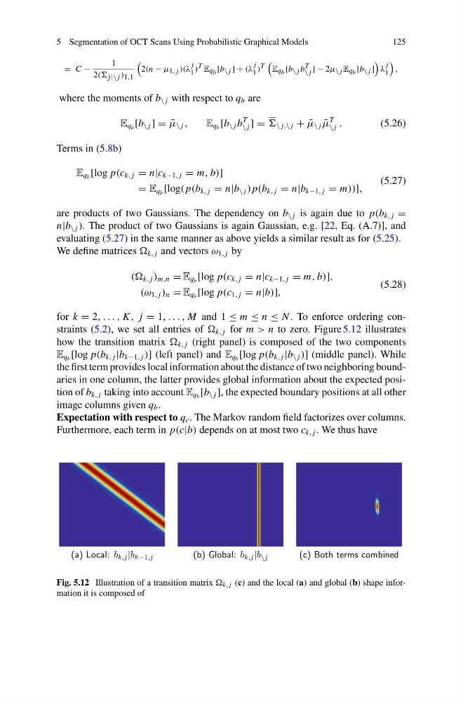
for k = 2, . . . , K , j = 1, . . . , M and 1 ≤ m ≤ n ≤ N . To enforce ordering constraints (5.2), we set all entries of k, j for m > n to zero. Figure 5.12 illustrates
how the transition matrix k, j (right panel) is composed of the two components
E q b [log p(b k, j |b k−1, j )] (left panel) and E q b [log p(b k, j |b \ j )] (middle panel). While
the first term provides local information about the distance of two neighboring boundaries in one column, the latter provides global information about the expected position of b k, j taking into account E q b [b \ j ], the expected boundary positions at all other
image columns given q b .
Expectation with respect to q c . The Markov random field factorizes over columns.
Furthermore, each term in p(c|b) depends on at most two c k, j . We thus have
(a) Local: b k,j |b k−1,j
(b) Global: b k,j |b \j
(c) Both terms combined
Fig. 5.12 Illustration of a transition matrix k, j (c) and the local (a) and global (b) shape information it is composed of
125
= C −
1
2(( j|\ j ) 1,1
2(n − μ 1, j )(λ
j
1 ) T E q b [b \ j ] + (λ
j
1 ) T
E q b [b \ j b T
\ j ] − 2μ \ j E q b [b \ j ]
λ
j
1
,
where the moments of b \ j with respect to q b are
E q b [b \ j ] = ¯
μ \ j ,
E q b [b \ j b
T
\ j ] = \ j,\ j + ¯
μ \ j ¯
μ
T
\ j .
(5.26)
Terms in (5.8b)
E q b [log p(c k, j = n|c k−1, j = m, b)]
= E q b [log( p(b k, j = n|b \ j ) p(b k, j = n|b k−1, j = m))],
(5.27)
are products of two Gaussians. The dependency on b \ j is again due to p(b k, j =
n|b \ j ). The product of two Gaussians is again Gaussian, e.g. [22, Eq. (A.7)], and
evaluating (5.27) in the same manner as above yields a similar result as for (5.25).
We define matrices k, j and vectors ω 1, j by
(( k, j ) m,n = E q b [log p(c k, j = n|c k−1, j = m, b)],
(ω 1, j ) n = E q b [log p(c 1, j = n|b)],
(5.28)
for k = 2, . . . , K , j = 1, . . . , M and 1 ≤ m ≤ n ≤ N . To enforce ordering constraints (5.2), we set all entries of k, j for m > n to zero. Figure 5.12 illustrates
how the transition matrix k, j (right panel) is composed of the two components
E q b [log p(b k, j |b k−1, j )] (left panel) and E q b [log p(b k, j |b \ j )] (middle panel). While
the first term provides local information about the distance of two neighboring boundaries in one column, the latter provides global information about the expected position of b k, j taking into account E q b [b \ j ], the expected boundary positions at all other
image columns given q b .
Expectation with respect to q c . The Markov random field factorizes over columns.
Furthermore, each term in p(c|b) depends on at most two c k, j . We thus have
(a) Local: b k,j |b k−1,j
(b) Global: b k,j |b \j
(c) Both terms combined
Fig. 5.12 Illustration of a transition matrix k, j (c) and the local (a) and global (b) shape information it is composed of