

5 Segmentation of OCT Scans Using Probabilistic Graphical Models
121
Here subscripts a, b indicate the truncation of W to entries of columns between
a and b. Truncating the modes in W corresponds to taking the marginal Gaussian
model over the corresponding area. Also, note that the subscript 1, b − a indicates
the translation invariance of our pathological shape modifications.
Now, let L a,b (θ
l
a,b ) be the log-probability of the retina segmentation for region
[a, b] for some l ∈ {healthy, ill 1 , ill 2 , . . . , ill I }:
L a,b (θ
l
a,b ) := log q
c a,b , b a,b |θ
l
a,b
.
(5.17)
Here we made explicit the dependency on θ
l
a,b of q. Furthermore, let X = {x 1 , x 2 , ...,
x K , M} denote the partition of the M columns into K + 1 regions, and let θ =
{θ
l 1
1,x 1
, θ
l 2
x 1 ,x 2
, . . . , θ
l K
x K ,M } denote a corresponding set of modified shape priors. Then,
exploiting the independence property, the log-probability for the full scan can be
written as sum of local terms:
L 1,M (θ, X, K ) = L 1,x 1 (θ
l 1
1,x 2
) + L x 1 ,x 2 (θ
l 2
x 1 ,x 2
) + . . . + L x K ,M (θ
l K
x K ,M ).
(5.18)
Maximum Likelihood. The objective is to find the optimal combination of regions
and corresponding priors θ :
max
K
max
X
max
θ
L 1,M (θ, X, K ).
(5.19)
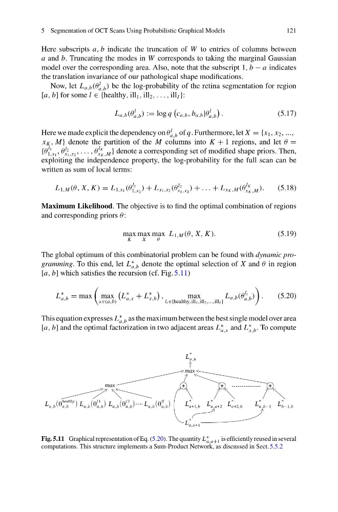
The global optimum of this combinatorial problem can be found with dynamic programming. To this end, let L
∗
a,b denote the optimal selection of X and θ in region
[a, b] which satisfies the recursion (cf. Fig. 5.11)
L
∗
a,b = max
max
x∈(a,b)
L
∗
a,x + L
∗
x,b
,
max
l i ∈{healthy,ill 1 ,ill 2 ,...,ill I }
L a,b (θ
l i
a,b )
.
(5.20)
This equation expresses L
∗
a,b as the maximum between the best single model over area
[a, b] and the optimal factorization in two adjacent areas L
∗
a,x and L
∗
x,b . To compute
Fig. 5.11 Graphical representation of Eq. (5.20). The quantity L ∗
a,a+1 is efficiently reused in several
computations. This structure implements a Sum-Product Network, as discussed in Sect. 5.5.2
121
Here subscripts a, b indicate the truncation of W to entries of columns between
a and b. Truncating the modes in W corresponds to taking the marginal Gaussian
model over the corresponding area. Also, note that the subscript 1, b − a indicates
the translation invariance of our pathological shape modifications.
Now, let L a,b (θ
l
a,b ) be the log-probability of the retina segmentation for region
[a, b] for some l ∈ {healthy, ill 1 , ill 2 , . . . , ill I }:
L a,b (θ
l
a,b ) := log q
c a,b , b a,b |θ
l
a,b
.
(5.17)
Here we made explicit the dependency on θ
l
a,b of q. Furthermore, let X = {x 1 , x 2 , ...,
x K , M} denote the partition of the M columns into K + 1 regions, and let θ =
{θ
l 1
1,x 1
, θ
l 2
x 1 ,x 2
, . . . , θ
l K
x K ,M } denote a corresponding set of modified shape priors. Then,
exploiting the independence property, the log-probability for the full scan can be
written as sum of local terms:
L 1,M (θ, X, K ) = L 1,x 1 (θ
l 1
1,x 2
) + L x 1 ,x 2 (θ
l 2
x 1 ,x 2
) + . . . + L x K ,M (θ
l K
x K ,M ).
(5.18)
Maximum Likelihood. The objective is to find the optimal combination of regions
and corresponding priors θ :
max
K
max
X
max
θ
L 1,M (θ, X, K ).
(5.19)
The global optimum of this combinatorial problem can be found with dynamic programming. To this end, let L
∗
a,b denote the optimal selection of X and θ in region
[a, b] which satisfies the recursion (cf. Fig. 5.11)
L
∗
a,b = max
max
x∈(a,b)
L
∗
a,x + L
∗
x,b
,
max
l i ∈{healthy,ill 1 ,ill 2 ,...,ill I }
L a,b (θ
l i
a,b )
.
(5.20)
This equation expresses L
∗
a,b as the maximum between the best single model over area
[a, b] and the optimal factorization in two adjacent areas L
∗
a,x and L
∗
x,b . To compute
Fig. 5.11 Graphical representation of Eq. (5.20). The quantity L ∗
a,a+1 is efficiently reused in several
computations. This structure implements a Sum-Product Network, as discussed in Sect. 5.5.2