4.5.2
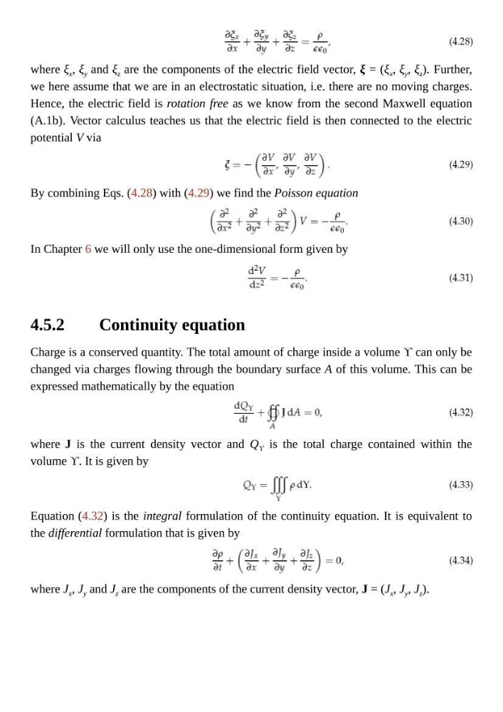
where ξ x , ξ y and ξ z are the components of the electric field vector, ξ = (ξ x , ξ y , ξ z ). Further,
we here assume that we are in an electrostatic situation, i.e. there are no moving charges.
Hence, the electric field is rotation free as we know from the second Maxwell equation
(A.1b). Vector calculus teaches us that the electric field is then connected to the electric
potential V via
By combining Eqs. (4.28) with (4.29) we find the Poisson equation
In Chapter 6 we will only use the one-dimensional form given by
Continuity equation
Charge is a conserved quantity. The total amount of charge inside a volume ϒ can only be
changed via charges flowing through the boundary surface A of this volume. This can be
expressed mathematically by the equation
where J is the current density vector and Q ϒ is the total charge contained within the
volume ϒ. It is given by
Equation (4.32) is the integral formulation of the continuity equation. It is equivalent to
the differential formulation that is given by
where J x , J y and J z are the components of the current density vector, J = (J x , J y , J z ).