

Can Quantum Theory Concepts Shed Light on Biological Evolution Processes?
455
same remarks apply as to the successive levels of organization, from biopolymers to
ecosystems. Now we have to relate the requirements expressed in Eqs. (12) and (13).
On one hand, it is known from numerous examples [3–11] that, when submitted to
natural selection under changing environment, a species has better chance to survive
when it shows more varieties, more overall complexity. This means that ‘complexity’
is, as least for species, and also partly for individuals, a general condition for ‘fitness’.
But the increase of complexity is also, as we saw in §4.1, a general trend in Nature.
The natural trend then seems to be not ‘complexity for fitness’ (there are many other
conditions for fitness), but rather ‘fitness-selected complexity’ (from an interplay
between ‘chance and necessity’). Assuming there is ‘complexification’ from t a to t
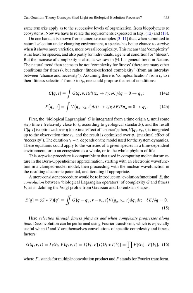
then ‘fitness selection’ from t to t b , one could propose the set of conditions:
C[q, t] ≡
G(q, v, t)dt(t a → t); δC/δq = 0 → q o ;
(14a)
F
q o , t
≡
V
q o , v o , t
dt(t → t b ); δ F/δq o = 0 → q r .
(14b)
First, the ‘biological Lagrangian’ G is integrated from a time origin t a until some
step time t (relatively close to t a according to geological standards), and the result
C[q, t] is optimized over q (maximal effect of ‘chance’); then, V [q o , v o , t] is integrated
up to the observation time t b , and the result is optimized over q o (maximal effect of
‘necessity’). The duration t b − t a depends on the model used for the system dynamics.
These equations could apply to the varieties of a given species in a time-dependent
environment, or to an ecosystem as a whole, or to the whole phylum of life.
This stepwise procedure is comparable to that used in computing molecular structure in the Born-Oppenheimer approximation, starting with an electronic wavefunction in a clamped-nuclei model, then proceeding with the nuclear wavefunction in
the resulting electronic potential, and iterating if appropriate.
A more consistent procedure would be to introduce an ‘evolution functional’ E, the
convolution between ‘biological Lagrangian operators’ of complexity G and fitness
V, as in defining the Voigt profile from Gaussian and Lorentzian shapes:
E[q] ≡ (G ∗ V )[q] ≡
¨
G
q − q a , v − v a , t
V
q a , v a , t
dq a dt; δ E/δq = 0.
(15)
Here selection through fitness plays as and when complexity progresses along
time. Deconvolution can be performed using Fourier transforms, which is especially
useful when G and V are themselves convolutions of specific complexity and fitness
factors:
G(q, v, t) = Γ i G i , V (q, v, t) = Γ i V i ; F[Γ i G i ∗ Γ i V i ] =
i
F[G i ] · F[V i ], (16)
where Γ i stands for multiple convolution product and F stands for Fourier transform.
455
same remarks apply as to the successive levels of organization, from biopolymers to
ecosystems. Now we have to relate the requirements expressed in Eqs. (12) and (13).
On one hand, it is known from numerous examples [3–11] that, when submitted to
natural selection under changing environment, a species has better chance to survive
when it shows more varieties, more overall complexity. This means that ‘complexity’
is, as least for species, and also partly for individuals, a general condition for ‘fitness’.
But the increase of complexity is also, as we saw in §4.1, a general trend in Nature.
The natural trend then seems to be not ‘complexity for fitness’ (there are many other
conditions for fitness), but rather ‘fitness-selected complexity’ (from an interplay
between ‘chance and necessity’). Assuming there is ‘complexification’ from t a to t
then ‘fitness selection’ from t to t b , one could propose the set of conditions:
C[q, t] ≡
G(q, v, t)dt(t a → t); δC/δq = 0 → q o ;
(14a)
F
q o , t
≡
V
q o , v o , t
dt(t → t b ); δ F/δq o = 0 → q r .
(14b)
First, the ‘biological Lagrangian’ G is integrated from a time origin t a until some
step time t (relatively close to t a according to geological standards), and the result
C[q, t] is optimized over q (maximal effect of ‘chance’); then, V [q o , v o , t] is integrated
up to the observation time t b , and the result is optimized over q o (maximal effect of
‘necessity’). The duration t b − t a depends on the model used for the system dynamics.
These equations could apply to the varieties of a given species in a time-dependent
environment, or to an ecosystem as a whole, or to the whole phylum of life.
This stepwise procedure is comparable to that used in computing molecular structure in the Born-Oppenheimer approximation, starting with an electronic wavefunction in a clamped-nuclei model, then proceeding with the nuclear wavefunction in
the resulting electronic potential, and iterating if appropriate.
A more consistent procedure would be to introduce an ‘evolution functional’ E, the
convolution between ‘biological Lagrangian operators’ of complexity G and fitness
V, as in defining the Voigt profile from Gaussian and Lorentzian shapes:
E[q] ≡ (G ∗ V )[q] ≡
¨
G
q − q a , v − v a , t
V
q a , v a , t
dq a dt; δ E/δq = 0.
(15)
Here selection through fitness plays as and when complexity progresses along
time. Deconvolution can be performed using Fourier transforms, which is especially
useful when G and V are themselves convolutions of specific complexity and fitness
factors:
G(q, v, t) = Γ i G i , V (q, v, t) = Γ i V i ; F[Γ i G i ∗ Γ i V i ] =
i
F[G i ] · F[V i ], (16)
where Γ i stands for multiple convolution product and F stands for Fourier transform.