

Abiogenesis and the Second Law of Thermodynamics
423
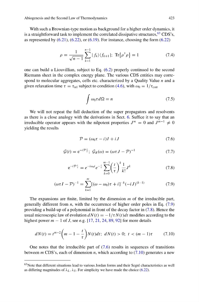
With such a Brownian-type motion as background for a higher order dynamics, it
is a straightforward task to implement the correlated dissipative structures,
63 CDS’s,
as represented by (6.21), (6.22), or (6.19). For instance, choosing the form (6.22)
ρ =
1
√
n − 1
n−1
k=1
| f k f k+1 |; Tr
ρ
†
ρ
= 1
( 7 . 4 )
one can build a Liouvillian, subject to Eq. (6.2) properly continued to the second
Riemann sheet in the complex energy plane. The various CDS entities may correspond to molecular aggregates, cells etc. characterized by a Quality Value n and a
given relaxation time τ = τ rel subject to condition (4.6), with ω 0 = 1/τ corr
ω 0 τ d = n
(7.5)
We will not repeat the full deduction of the super propagators and resolvents
as there is a close analogy with the derivations in Sect. 6. Suffice it to say that an
irreducible operator appears with the nilpotent properties J
m
= 0 and J
m−1
= 0
yielding the results
P = (ω 0 τ − i)I + i J
(7.6)
G(t) = e
−iP
t
τ ; G R (ω) = (ωτ J − P)
−1
(7.7)
e
−iP
t
τ = e
−iω 0 t e
−
t
τ
m−1
k=0
t
τ
k 1
k!
J
k
(7.8)
(ωτ I − P)
−1
=
m
k=1
[(ω − ω 0 )τ + i]
−k
(−i J )
(k−1)
(7.9)
The expansions are finite, limited by the dimension m of the irreducible part,
generally different from n, with the occurrence of higher order poles in Eq. (7.9)
providing a build-up of a polynomial in front of the decay factor in (7.8). Hence the
usual microscopic law of evolution d N (t) = −1/τ N (t)dt modifies according to the
highest power m − 1 of J, see e.g. [17, 21, 24, 89, 92] for more details
d N (t) = t
m−2
m − 1 −
t
τ
N (t)dt; d N (t) > 0; t < (m − 1)τ
(7.10)
One notes that the irreducible part of (7.6) results in sequences of transitions
between m CDS’s, each of dimension n, which according to (7.10) generates a new
63 Note that different situations lead to various Jordan forms and their Segré characteristics as well
as differing magnitudes of λ L , λ S . For simplicity we have made the choice (6.22).
423
With such a Brownian-type motion as background for a higher order dynamics, it
is a straightforward task to implement the correlated dissipative structures,
63 CDS’s,
as represented by (6.21), (6.22), or (6.19). For instance, choosing the form (6.22)
ρ =
1
√
n − 1
n−1
k=1
| f k f k+1 |; Tr
ρ
†
ρ
= 1
( 7 . 4 )
one can build a Liouvillian, subject to Eq. (6.2) properly continued to the second
Riemann sheet in the complex energy plane. The various CDS entities may correspond to molecular aggregates, cells etc. characterized by a Quality Value n and a
given relaxation time τ = τ rel subject to condition (4.6), with ω 0 = 1/τ corr
ω 0 τ d = n
(7.5)
We will not repeat the full deduction of the super propagators and resolvents
as there is a close analogy with the derivations in Sect. 6. Suffice it to say that an
irreducible operator appears with the nilpotent properties J
m
= 0 and J
m−1
= 0
yielding the results
P = (ω 0 τ − i)I + i J
(7.6)
G(t) = e
−iP
t
τ ; G R (ω) = (ωτ J − P)
−1
(7.7)
e
−iP
t
τ = e
−iω 0 t e
−
t
τ
m−1
k=0
t
τ
k 1
k!
J
k
(7.8)
(ωτ I − P)
−1
=
m
k=1
[(ω − ω 0 )τ + i]
−k
(−i J )
(k−1)
(7.9)
The expansions are finite, limited by the dimension m of the irreducible part,
generally different from n, with the occurrence of higher order poles in Eq. (7.9)
providing a build-up of a polynomial in front of the decay factor in (7.8). Hence the
usual microscopic law of evolution d N (t) = −1/τ N (t)dt modifies according to the
highest power m − 1 of J, see e.g. [17, 21, 24, 89, 92] for more details
d N (t) = t
m−2
m − 1 −
t
τ
N (t)dt; d N (t) > 0; t < (m − 1)τ
(7.10)
One notes that the irreducible part of (7.6) results in sequences of transitions
between m CDS’s, each of dimension n, which according to (7.10) generates a new
63 Note that different situations lead to various Jordan forms and their Segré characteristics as well
as differing magnitudes of λ L , λ S . For simplicity we have made the choice (6.22).