

328
M. Svrˇ cek
set of fermionic and bosonic operators, with the transformed Hamiltonian optimized
on the Born-Oppenheimer (B-O) level for adiabatic molecules.
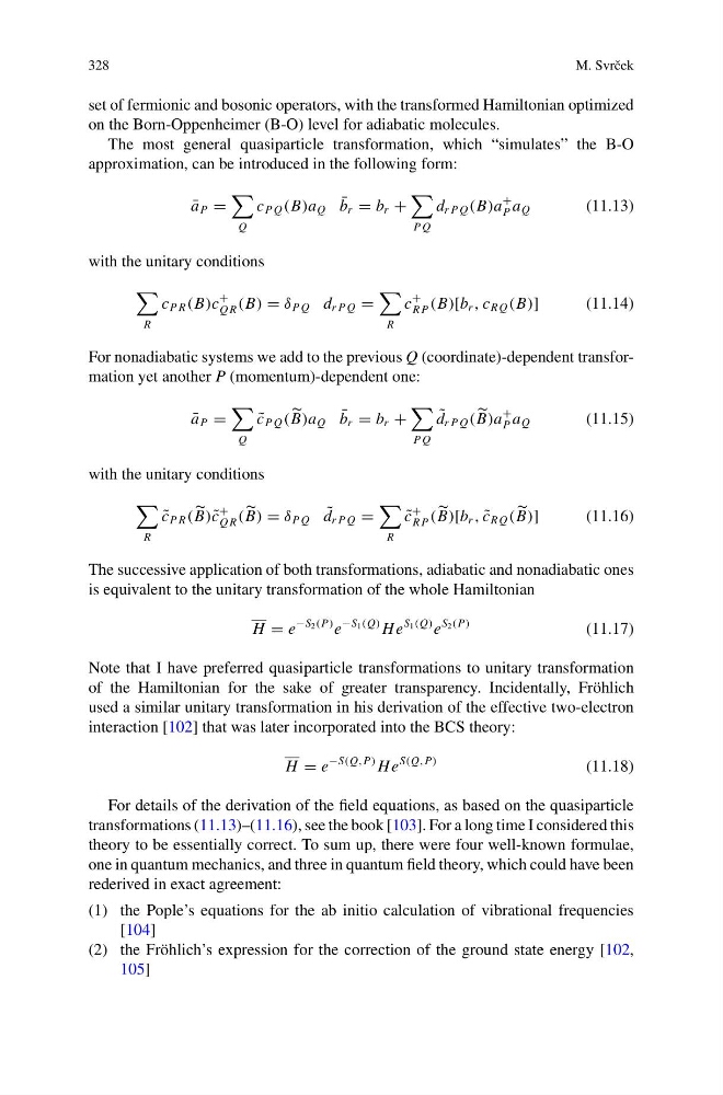
The most general quasiparticle transformation, which “simulates” the B-O
approximation, can be introduced in the following form:
¯
a P =
Q
c P Q (B)a Q ¯
b r = b r +
P Q
d r P Q (B)a
+
P a Q
(11.13)
with the unitary conditions
R
c P R (B)c
+
Q R (B) = δ P Q d r P Q =
R
c
+
R P (B)[b r , c R Q (B)]
(11.14)
For nonadiabatic systems we add to the previous Q (coordinate)-dependent transformation yet another P (momentum)-dependent one:
¯
a P =
Q
˜
c P Q ( B)a Q ¯
b r = b r +
P Q
˜
d r P Q ( B)a
+
P a Q
(11.15)
with the unitary conditions
R
˜
c P R ( B) ˜
c
+
Q R ( B) = δ P Q ˜
d r P Q =
R
˜
c
+
R P ( B)[b r , ˜
c R Q ( B)]
(11.16)
The successive application of both transformations, adiabatic and nonadiabatic ones
is equivalent to the unitary transformation of the whole Hamiltonian
H = e
−S 2 (P) e
−S 1 (Q) He
S 1 (Q) e
S 2 (P)
(11.17)
Note that I have preferred quasiparticle transformations to unitary transformation
of the Hamiltonian for the sake of greater transparency. Incidentally, Fröhlich
used a similar unitary transformation in his derivation of the effective two-electron
interaction [102] that was later incorporated into the BCS theory:
H = e
−S(Q,P) He
S(Q,P)
(11.18)
For details of the derivation of the field equations, as based on the quasiparticle
transformations (11.13)–(11.16), see the book [103]. For a long time I considered this
theory to be essentially correct. To sum up, there were four well-known formulae,
one in quantum mechanics, and three in quantum field theory, which could have been
rederived in exact agreement:
(1) the Pople’s equations for the ab initio calculation of vibrational frequencies
[104]
(2) the Fröhlich’s expression for the correction of the ground state energy [102,
105]
M. Svrˇ cek
set of fermionic and bosonic operators, with the transformed Hamiltonian optimized
on the Born-Oppenheimer (B-O) level for adiabatic molecules.
The most general quasiparticle transformation, which “simulates” the B-O
approximation, can be introduced in the following form:
¯
a P =
Q
c P Q (B)a Q ¯
b r = b r +
P Q
d r P Q (B)a
+
P a Q
(11.13)
with the unitary conditions
R
c P R (B)c
+
Q R (B) = δ P Q d r P Q =
R
c
+
R P (B)[b r , c R Q (B)]
(11.14)
For nonadiabatic systems we add to the previous Q (coordinate)-dependent transformation yet another P (momentum)-dependent one:
¯
a P =
Q
˜
c P Q ( B)a Q ¯
b r = b r +
P Q
˜
d r P Q ( B)a
+
P a Q
(11.15)
with the unitary conditions
R
˜
c P R ( B) ˜
c
+
Q R ( B) = δ P Q ˜
d r P Q =
R
˜
c
+
R P ( B)[b r , ˜
c R Q ( B)]
(11.16)
The successive application of both transformations, adiabatic and nonadiabatic ones
is equivalent to the unitary transformation of the whole Hamiltonian
H = e
−S 2 (P) e
−S 1 (Q) He
S 1 (Q) e
S 2 (P)
(11.17)
Note that I have preferred quasiparticle transformations to unitary transformation
of the Hamiltonian for the sake of greater transparency. Incidentally, Fröhlich
used a similar unitary transformation in his derivation of the effective two-electron
interaction [102] that was later incorporated into the BCS theory:
H = e
−S(Q,P) He
S(Q,P)
(11.18)
For details of the derivation of the field equations, as based on the quasiparticle
transformations (11.13)–(11.16), see the book [103]. For a long time I considered this
theory to be essentially correct. To sum up, there were four well-known formulae,
one in quantum mechanics, and three in quantum field theory, which could have been
rederived in exact agreement:
(1) the Pople’s equations for the ab initio calculation of vibrational frequencies
[104]
(2) the Fröhlich’s expression for the correction of the ground state energy [102,
105]