

322
M. Svrˇ cek
F
μν
≡ ∂
μ A
ν
− ∂
ν A
μ
; D μ ≡ ∂ μ + iq A μ
(10.9)
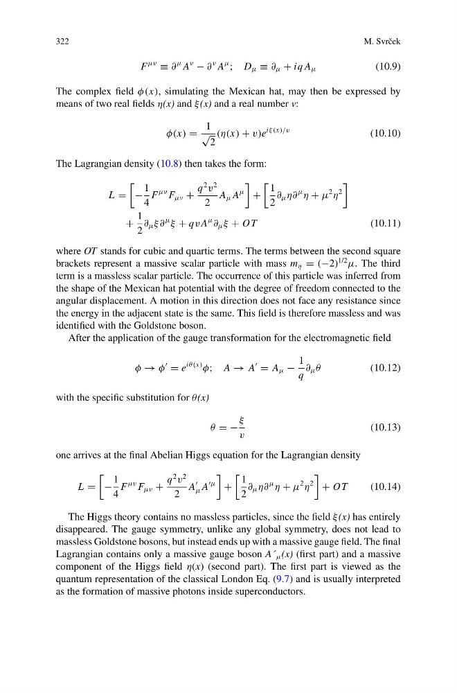
The complex field φ(x), simulating the Mexican hat, may then be expressed by
means of two real fields η(x) and ξ (x) and a real number v:
φ(x) =
1
√
2
(η(x) + v)e
iξ (x)/v
(10.10)
The Lagrangian density (10.8) then takes the form:
L =
−
1
4
F
μν F μν +
q
2
v
2
2
A μ A
μ
+
1
2
∂ μ η∂
μ
η + μ
2
η
2
+
1
2
∂ μ ξ∂
μ
ξ + qv A
μ
∂ μ ξ + OT
(10.11)
where OT stands for cubic and quartic terms. The terms between the second square
brackets represent a massive scalar particle with mass m η = (−2)
1/2
μ. The third
term is a massless scalar particle. The occurrence of this particle was inferred from
the shape of the Mexican hat potential with the degree of freedom connected to the
angular displacement. A motion in this direction does not face any resistance since
the energy in the adjacent state is the same. This field is therefore massless and was
identified with the Goldstone boson.
After the application of the gauge transformation for the electromagnetic field
φ → φ
= e
iθ(x)
φ; A → A
= A μ −
1
q
∂ μ θ
(10.12)
with the specific substitution for θ (x)
θ = −
ξ
v
(10.13)
one arrives at the final Abelian Higgs equation for the Lagrangian density
L =
−
1
4
F
μν F μν +
q
2
v
2
2
A
μ A
μ
+
1
2
∂ μ η∂
μ
η + μ
2
η
2
+ OT
(10.14)
The Higgs theory contains no massless particles, since the field ξ (x) has entirely
disappeared. The gauge symmetry, unlike any global symmetry, does not lead to
massless Goldstone bosons, but instead ends up with a massive gauge field. The final
Lagrangian contains only a massive gauge boson A´ μ (x) (first part) and a massive
component of the Higgs field η(x) (second part). The first part is viewed as the
quantum representation of the classical London Eq. (9.7) and is usually interpreted
as the formation of massive photons inside superconductors.
M. Svrˇ cek
F
μν
≡ ∂
μ A
ν
− ∂
ν A
μ
; D μ ≡ ∂ μ + iq A μ
(10.9)
The complex field φ(x), simulating the Mexican hat, may then be expressed by
means of two real fields η(x) and ξ (x) and a real number v:
φ(x) =
1
√
2
(η(x) + v)e
iξ (x)/v
(10.10)
The Lagrangian density (10.8) then takes the form:
L =
−
1
4
F
μν F μν +
q
2
v
2
2
A μ A
μ
+
1
2
∂ μ η∂
μ
η + μ
2
η
2
+
1
2
∂ μ ξ∂
μ
ξ + qv A
μ
∂ μ ξ + OT
(10.11)
where OT stands for cubic and quartic terms. The terms between the second square
brackets represent a massive scalar particle with mass m η = (−2)
1/2
μ. The third
term is a massless scalar particle. The occurrence of this particle was inferred from
the shape of the Mexican hat potential with the degree of freedom connected to the
angular displacement. A motion in this direction does not face any resistance since
the energy in the adjacent state is the same. This field is therefore massless and was
identified with the Goldstone boson.
After the application of the gauge transformation for the electromagnetic field
φ → φ
= e
iθ(x)
φ; A → A
= A μ −
1
q
∂ μ θ
(10.12)
with the specific substitution for θ (x)
θ = −
ξ
v
(10.13)
one arrives at the final Abelian Higgs equation for the Lagrangian density
L =
−
1
4
F
μν F μν +
q
2
v
2
2
A
μ A
μ
+
1
2
∂ μ η∂
μ
η + μ
2
η
2
+ OT
(10.14)
The Higgs theory contains no massless particles, since the field ξ (x) has entirely
disappeared. The gauge symmetry, unlike any global symmetry, does not lead to
massless Goldstone bosons, but instead ends up with a massive gauge field. The final
Lagrangian contains only a massive gauge boson A´ μ (x) (first part) and a massive
component of the Higgs field η(x) (second part). The first part is viewed as the
quantum representation of the classical London Eq. (9.7) and is usually interpreted
as the formation of massive photons inside superconductors.