

Advanced Relativistic Energy Approach in Spectroscopy …
15
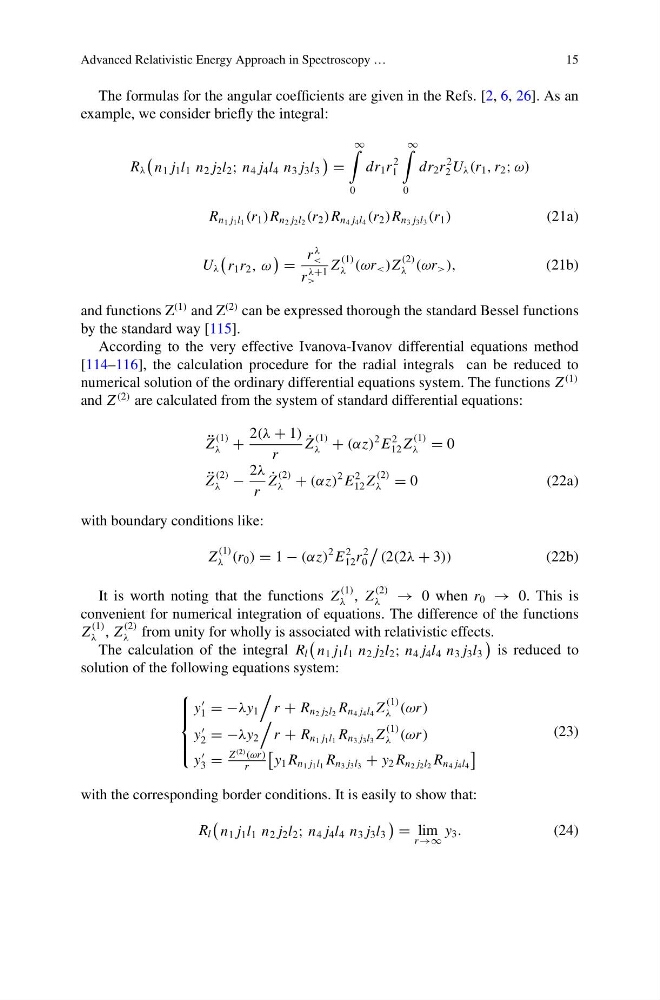
The formulas for the angular coefficients are given in the Refs. [2, 6, 26]. As an
example, we consider briefly the integral:
R λ
n 1 j 1 l 1 n 2 j 2 l 2 ; n 4 j 4 l 4 n 3 j 3 l 3
=
∞
0
dr 1 r
2
1
∞
0
dr 2 r
2
2 U λ (r 1 , r 2 ; ω)
R n 1 j 1 l 1 (r 1 )R n 2 j 2 l 2 (r 2 )R n 4 j 4 l 4 (r 2 )R n 3 j 3 l 3 (r 1 )
(21a)
U λ
r 1 r 2 , ω
=
r
λ
<
r
λ+1
>
Z
(1)
λ (ωr < )Z
(2)
λ (ωr > ),
(21b)
and functions Z
(1) and Z
(2) can be expressed thorough the standard Bessel functions
by the standard way [115].
According to the very effective Ivanova-Ivanov differential equations method
[114–116], the calculation procedure for the radial integrals can be reduced to
numerical solution of the ordinary differential equations system. The functions Z
(1)
and Z
(2) are calculated from the system of standard differential equations:
¨
Z
(1)
λ +
2(λ + 1)
r
˙
Z
(1)
λ + (αz)
2 E
2
12 Z
(1)
λ = 0
¨
Z
(2)
λ −
2λ
r
˙
Z
(2)
λ + (αz)
2 E
2
12 Z
(2)
λ = 0
(22a)
with boundary conditions like:
Z
(1)
λ (r 0 ) = 1 − (αz)
2 E
2
12 r
2
0
(2(2λ + 3))
(22b)
It is worth noting that the functions Z
(1)
λ , Z
(2)
λ
→ 0 when r 0 → 0. This is
convenient for numerical integration of equations. The difference of the functions
Z
(1)
λ , Z
(2)
λ from unity for wholly is associated with relativistic effects.
The calculation of the integral R l
n 1 j 1 l 1 n 2 j 2 l 2 ; n 4 j 4 l 4 n 3 j 3 l 3
is reduced to
solution of the following equations system:
⎧
⎪ ⎪ ⎨
⎪ ⎪ ⎩
y
1 = −λy 1
r + R n 2 j 2 l 2 R n 4 j 4 l 4 Z
(1)
λ (ωr )
y
2 = −λy 2
r + R n 1 j 1 l 1 R n 3 j 3 l 3 Z
(1)
λ (ωr )
y
3 =
Z
(2) (ωr )
r
y 1 R n 1 j 1 l 1 R n 3 j 3 l 3 + y 2 R n 2 j 2 l 2 R n 4 j 4 l 4
(23)
with the corresponding border conditions. It is easily to show that:
R l
n 1 j 1 l 1 n 2 j 2 l 2 ; n 4 j 4 l 4 n 3 j 3 l 3
= lim
r →∞
y 3 .
(24)
15
The formulas for the angular coefficients are given in the Refs. [2, 6, 26]. As an
example, we consider briefly the integral:
R λ
n 1 j 1 l 1 n 2 j 2 l 2 ; n 4 j 4 l 4 n 3 j 3 l 3
=
∞
0
dr 1 r
2
1
∞
0
dr 2 r
2
2 U λ (r 1 , r 2 ; ω)
R n 1 j 1 l 1 (r 1 )R n 2 j 2 l 2 (r 2 )R n 4 j 4 l 4 (r 2 )R n 3 j 3 l 3 (r 1 )
(21a)
U λ
r 1 r 2 , ω
=
r
λ
<
r
λ+1
>
Z
(1)
λ (ωr < )Z
(2)
λ (ωr > ),
(21b)
and functions Z
(1) and Z
(2) can be expressed thorough the standard Bessel functions
by the standard way [115].
According to the very effective Ivanova-Ivanov differential equations method
[114–116], the calculation procedure for the radial integrals can be reduced to
numerical solution of the ordinary differential equations system. The functions Z
(1)
and Z
(2) are calculated from the system of standard differential equations:
¨
Z
(1)
λ +
2(λ + 1)
r
˙
Z
(1)
λ + (αz)
2 E
2
12 Z
(1)
λ = 0
¨
Z
(2)
λ −
2λ
r
˙
Z
(2)
λ + (αz)
2 E
2
12 Z
(2)
λ = 0
(22a)
with boundary conditions like:
Z
(1)
λ (r 0 ) = 1 − (αz)
2 E
2
12 r
2
0
(2(2λ + 3))
(22b)
It is worth noting that the functions Z
(1)
λ , Z
(2)
λ
→ 0 when r 0 → 0. This is
convenient for numerical integration of equations. The difference of the functions
Z
(1)
λ , Z
(2)
λ from unity for wholly is associated with relativistic effects.
The calculation of the integral R l
n 1 j 1 l 1 n 2 j 2 l 2 ; n 4 j 4 l 4 n 3 j 3 l 3
is reduced to
solution of the following equations system:
⎧
⎪ ⎪ ⎨
⎪ ⎪ ⎩
y
1 = −λy 1
r + R n 2 j 2 l 2 R n 4 j 4 l 4 Z
(1)
λ (ωr )
y
2 = −λy 2
r + R n 1 j 1 l 1 R n 3 j 3 l 3 Z
(1)
λ (ωr )
y
3 =
Z
(2) (ωr )
r
y 1 R n 1 j 1 l 1 R n 3 j 3 l 3 + y 2 R n 2 j 2 l 2 R n 4 j 4 l 4
(23)
with the corresponding border conditions. It is easily to show that:
R l
n 1 j 1 l 1 n 2 j 2 l 2 ; n 4 j 4 l 4 n 3 j 3 l 3
= lim
r →∞
y 3 .
(24)