

Basics of beam dynamics 19
M 2
M 21
M 1
1
1
′
2
2
′
beam
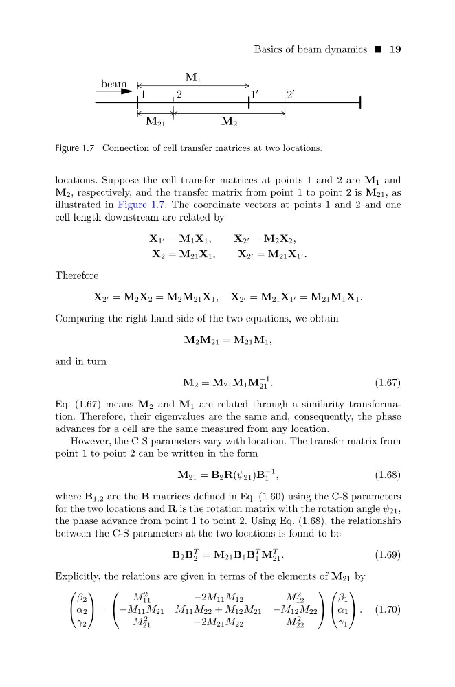
Figure 1.7 Connection of cell transfer matrices at two locations.
locations. Suppose the cell transfer matrices at points 1 and 2 are M 1 and
M 2 , respectively, and the transfer matrix from point 1 to point 2 is M 21 , as
illustrated in Figure 1.7. The coordinate vectors at points 1 and 2 and one
cell length downstream are related by
X 1 = M 1 X 1 ,
X 2 = M 2 X 2 ,
X 2 = M 21 X 1 ,
X 2 = M 21 X 1 .
Therefore
X 2 = M 2 X 2 = M 2 M 21 X 1 , X 2 = M 21 X 1 = M 21 M 1 X 1 .
Comparing the right hand side of the two equations, we obtain
M 2 M 21 = M 21 M 1 ,
and in turn
M 2 = M 21 M 1 M
−1
21 .
(1.67)
Eq. (1.67) means M 2 and M 1 are related through a similarity transformation. Therefore, their eigenvalues are the same and, consequently, the phase
advances for a cell are the same measured from any location.
However, the C-S parameters vary with location. The transfer matrix from
point 1 to point 2 can be written in the form
M 21 = B 2 R(ψ 21 )B
−1
1 ,
(1.68)
where B 1,2 are the B matrices defined in Eq. (1.60) using the C-S parameters
for the two locations and R is the rotation matrix with the rotation angle ψ 21 ,
the phase advance from point 1 to point 2. Using Eq. (1.68), the relationship
between the C-S parameters at the two locations is found to be
B 2 B
T
2 = M 21 B 1 B
T
1 M
T
21 .
(1.69)
Explicitly, the relations are given in terms of the elements of M 21 by
β 2
α 2
γ 2
=
M
2
11
−2M 11 M 12
M
2
12
−M 11 M 21 M 11 M 22 + M 12 M 21 −M 12 M 22
M
2
21
−2M 21 M 22
M
2
22
β 1
α 1
γ 1
. (1.70)
M 2
M 21
M 1
1
1
′
2
2
′
beam
Figure 1.7 Connection of cell transfer matrices at two locations.
locations. Suppose the cell transfer matrices at points 1 and 2 are M 1 and
M 2 , respectively, and the transfer matrix from point 1 to point 2 is M 21 , as
illustrated in Figure 1.7. The coordinate vectors at points 1 and 2 and one
cell length downstream are related by
X 1 = M 1 X 1 ,
X 2 = M 2 X 2 ,
X 2 = M 21 X 1 ,
X 2 = M 21 X 1 .
Therefore
X 2 = M 2 X 2 = M 2 M 21 X 1 , X 2 = M 21 X 1 = M 21 M 1 X 1 .
Comparing the right hand side of the two equations, we obtain
M 2 M 21 = M 21 M 1 ,
and in turn
M 2 = M 21 M 1 M
−1
21 .
(1.67)
Eq. (1.67) means M 2 and M 1 are related through a similarity transformation. Therefore, their eigenvalues are the same and, consequently, the phase
advances for a cell are the same measured from any location.
However, the C-S parameters vary with location. The transfer matrix from
point 1 to point 2 can be written in the form
M 21 = B 2 R(ψ 21 )B
−1
1 ,
(1.68)
where B 1,2 are the B matrices defined in Eq. (1.60) using the C-S parameters
for the two locations and R is the rotation matrix with the rotation angle ψ 21 ,
the phase advance from point 1 to point 2. Using Eq. (1.68), the relationship
between the C-S parameters at the two locations is found to be
B 2 B
T
2 = M 21 B 1 B
T
1 M
T
21 .
(1.69)
Explicitly, the relations are given in terms of the elements of M 21 by
β 2
α 2
γ 2
=
M
2
11
−2M 11 M 12
M
2
12
−M 11 M 21 M 11 M 22 + M 12 M 21 −M 12 M 22
M
2
21
−2M 21 M 22
M
2
22
β 1
α 1
γ 1
. (1.70)