

18 Beam-based Correction and Optimization for Accelerators
(a)
y
y
′
√
2βJ
√ 2γJ
slope=−
α
β
0
1
2
3
(b)
¯
y
¯
Py
0
1
2
3
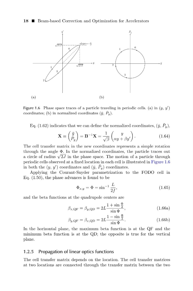
Figure 1.6 Phase space traces of a particle traveling in periodic cells. (a) in (y, y
)
coordinates; (b) in normalized coordinates (¯ y, ¯
Py).
Eq. (1.62) indicates that we can define the normalized coordinates, (¯ y, ¯
P y ),
¯
X ≡
¯
y
¯
P y
= B
−1 X =
1
√
β
y
αy + βy
.
(1.64)
The cell transfer matrix in the new coordinates represents a simple rotation
through the angle Φ. In the normalized coordinates, the particle traces out
a circle of radius
√
2J in the phase space. The motion of a particle through
periodic cells observed at a fixed location in each cell is illustrated in Figure 1.6
in both the (y, y
) coordinates and (¯ y, ¯
P y ) coordinates.
Applying the Courant-Snyder parametrization to the FODO cell in
Eq. (1.50), the phase advances is found to be
Φ x,y = Φ = sin
−1 L
2f
,
(1.65)
and the beta functions at the quadrupole centers are
β x,QF = β y,QD = 2L
1 + sin
Φ
2
sin Φ
,
(1.66a)
β y,QF = β x,QD = 2L
1 − sin
Φ
2
sin Φ
.
(1.66b)
In the horizontal plane, the maximum beta function is at the QF and the
minimum beta function is at the QD; the opposite is true for the vertical
plane.
1.2.5 Propagation of linear optics functions
The cell transfer matrix depends on the location. The cell transfer matrices
at two locations are connected through the transfer matrix between the two
(a)
y
y
′
√
2βJ
√ 2γJ
slope=−
α
β
0
1
2
3
(b)
¯
y
¯
Py
0
1
2
3
Figure 1.6 Phase space traces of a particle traveling in periodic cells. (a) in (y, y
)
coordinates; (b) in normalized coordinates (¯ y, ¯
Py).
Eq. (1.62) indicates that we can define the normalized coordinates, (¯ y, ¯
P y ),
¯
X ≡
¯
y
¯
P y
= B
−1 X =
1
√
β
y
αy + βy
.
(1.64)
The cell transfer matrix in the new coordinates represents a simple rotation
through the angle Φ. In the normalized coordinates, the particle traces out
a circle of radius
√
2J in the phase space. The motion of a particle through
periodic cells observed at a fixed location in each cell is illustrated in Figure 1.6
in both the (y, y
) coordinates and (¯ y, ¯
P y ) coordinates.
Applying the Courant-Snyder parametrization to the FODO cell in
Eq. (1.50), the phase advances is found to be
Φ x,y = Φ = sin
−1 L
2f
,
(1.65)
and the beta functions at the quadrupole centers are
β x,QF = β y,QD = 2L
1 + sin
Φ
2
sin Φ
,
(1.66a)
β y,QF = β x,QD = 2L
1 − sin
Φ
2
sin Φ
.
(1.66b)
In the horizontal plane, the maximum beta function is at the QF and the
minimum beta function is at the QD; the opposite is true for the vertical
plane.
1.2.5 Propagation of linear optics functions
The cell transfer matrix depends on the location. The cell transfer matrices
at two locations are connected through the transfer matrix between the two