

218 Beam-based Correction and Optimization for Accelerators
0
50
100
150
200
250
300
350
evaluation
0
0.2
0.4
0.6
x
-1.5
-1
-0.5
0
objective (mA/min)
RCDS
0
20
40
60
objective (um)
RCDS
0
50
100
150
200
250
evaluation
0.2
0.4
0.6
0.8
x
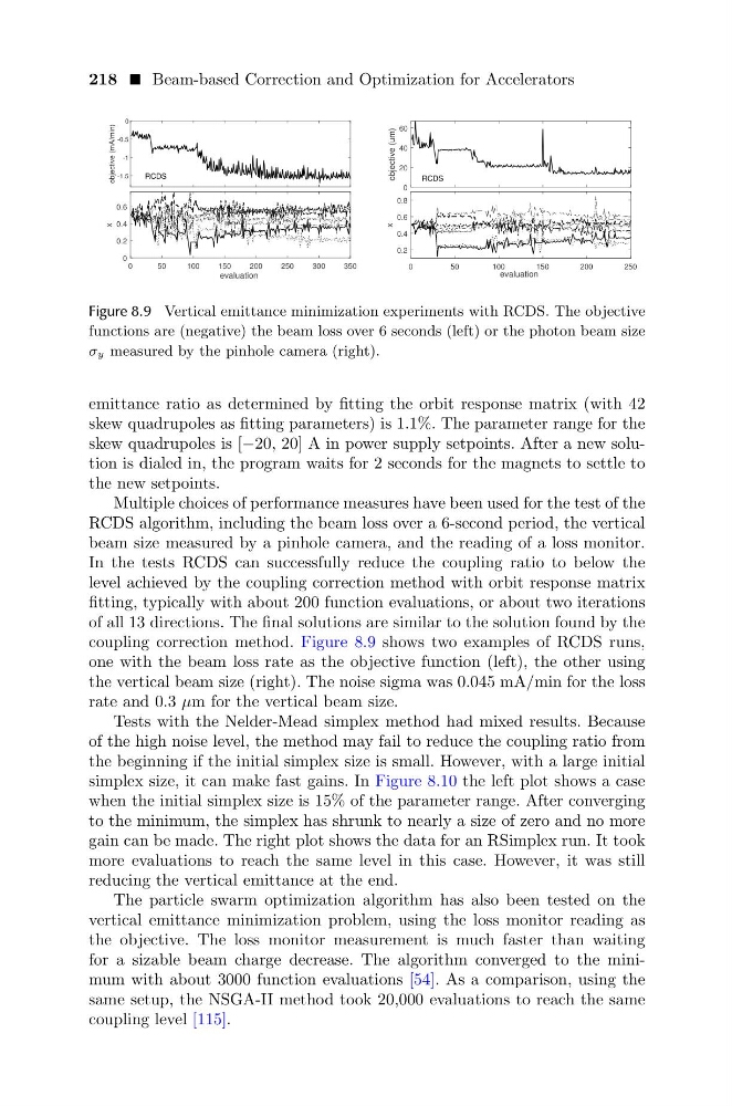
Figure 8.9 Vertical emittance minimization experiments with RCDS. The objective
functions are (negative) the beam loss over 6 seconds (left) or the photon beam size
σy measured by the pinhole camera (right).
emittance ratio as determined by fitting the orbit response matrix (with 42
skew quadrupoles as fitting parameters) is 1.1%. The parameter range for the
skew quadrupoles is [−20, 20] A in power supply setpoints. After a new solution is dialed in, the program waits for 2 seconds for the magnets to settle to
the new setpoints.
Multiple choices of performance measures have been used for the test of the
RCDS algorithm, including the beam loss over a 6-second period, the vertical
beam size measured by a pinhole camera, and the reading of a loss monitor.
In the tests RCDS can successfully reduce the coupling ratio to below the
level achieved by the coupling correction method with orbit response matrix
fitting, typically with about 200 function evaluations, or about two iterations
of all 13 directions. The final solutions are similar to the solution found by the
coupling correction method. Figure 8.9 shows two examples of RCDS runs,
one with the beam loss rate as the objective function (left), the other using
the vertical beam size (right). The noise sigma was 0.045 mA/min for the loss
rate and 0.3 µm for the vertical beam size.
Tests with the Nelder-Mead simplex method had mixed results. Because
of the high noise level, the method may fail to reduce the coupling ratio from
the beginning if the initial simplex size is small. However, with a large initial
simplex size, it can make fast gains. In Figure 8.10 the left plot shows a case
when the initial simplex size is 15% of the parameter range. After converging
to the minimum, the simplex has shrunk to nearly a size of zero and no more
gain can be made. The right plot shows the data for an RSimplex run. It took
more evaluations to reach the same level in this case. However, it was still
reducing the vertical emittance at the end.
The particle swarm optimization algorithm has also been tested on the
vertical emittance minimization problem, using the loss monitor reading as
the objective. The loss monitor measurement is much faster than waiting
for a sizable beam charge decrease. The algorithm converged to the minimum with about 3000 function evaluations [54]. As a comparison, using the
same setup, the NSGA-II method took 20,000 evaluations to reach the same
coupling level [115].
0
50
100
150
200
250
300
350
evaluation
0
0.2
0.4
0.6
x
-1.5
-1
-0.5
0
objective (mA/min)
RCDS
0
20
40
60
objective (um)
RCDS
0
50
100
150
200
250
evaluation
0.2
0.4
0.6
0.8
x
Figure 8.9 Vertical emittance minimization experiments with RCDS. The objective
functions are (negative) the beam loss over 6 seconds (left) or the photon beam size
σy measured by the pinhole camera (right).
emittance ratio as determined by fitting the orbit response matrix (with 42
skew quadrupoles as fitting parameters) is 1.1%. The parameter range for the
skew quadrupoles is [−20, 20] A in power supply setpoints. After a new solution is dialed in, the program waits for 2 seconds for the magnets to settle to
the new setpoints.
Multiple choices of performance measures have been used for the test of the
RCDS algorithm, including the beam loss over a 6-second period, the vertical
beam size measured by a pinhole camera, and the reading of a loss monitor.
In the tests RCDS can successfully reduce the coupling ratio to below the
level achieved by the coupling correction method with orbit response matrix
fitting, typically with about 200 function evaluations, or about two iterations
of all 13 directions. The final solutions are similar to the solution found by the
coupling correction method. Figure 8.9 shows two examples of RCDS runs,
one with the beam loss rate as the objective function (left), the other using
the vertical beam size (right). The noise sigma was 0.045 mA/min for the loss
rate and 0.3 µm for the vertical beam size.
Tests with the Nelder-Mead simplex method had mixed results. Because
of the high noise level, the method may fail to reduce the coupling ratio from
the beginning if the initial simplex size is small. However, with a large initial
simplex size, it can make fast gains. In Figure 8.10 the left plot shows a case
when the initial simplex size is 15% of the parameter range. After converging
to the minimum, the simplex has shrunk to nearly a size of zero and no more
gain can be made. The right plot shows the data for an RSimplex run. It took
more evaluations to reach the same level in this case. However, it was still
reducing the vertical emittance at the end.
The particle swarm optimization algorithm has also been tested on the
vertical emittance minimization problem, using the loss monitor reading as
the objective. The loss monitor measurement is much faster than waiting
for a sizable beam charge decrease. The algorithm converged to the minimum with about 3000 function evaluations [54]. As a comparison, using the
same setup, the NSGA-II method took 20,000 evaluations to reach the same
coupling level [115].