

160 Beam-based Correction and Optimization for Accelerators
10
-2
10
0
10
2
h
x
-
x
y
, f1001
1- x , f2000
0
0.2
0.4
0.6
0.8
1
tune
10
-2
10
0
10
2
h
y
-
y
x
, f0110
1- y , f0020
1- y , f1010
1- x , f1010
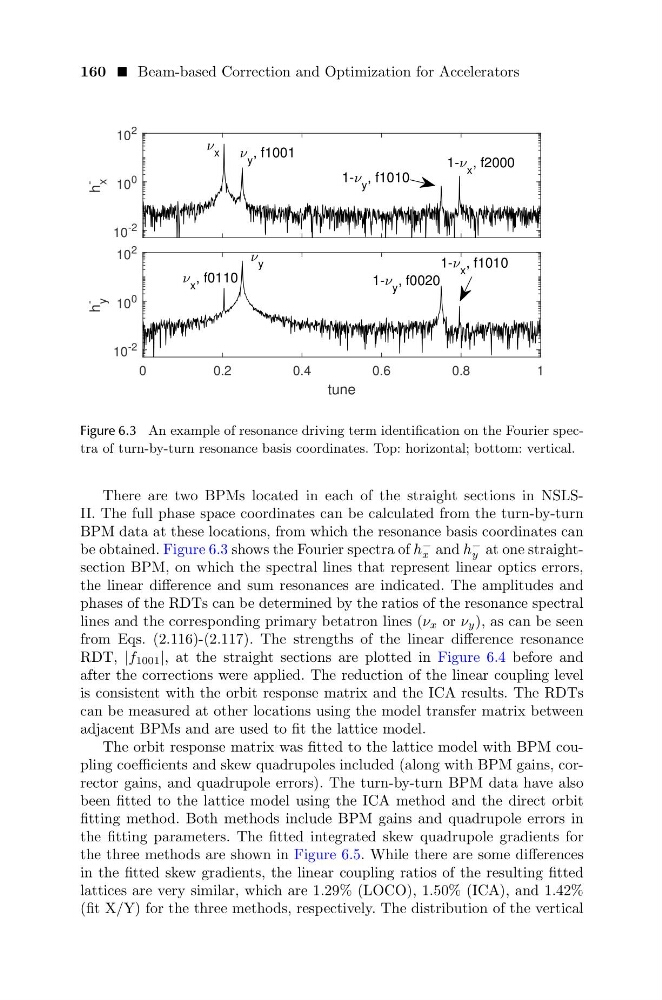
Figure 6.3 An example of resonance driving term identification on the Fourier spectra of turn-by-turn resonance basis coordinates. Top: horizontal; bottom: vertical.
There are two BPMs located in each of the straight sections in NSLSII. The full phase space coordinates can be calculated from the turn-by-turn
BPM data at these locations, from which the resonance basis coordinates can
be obtained. Figure 6.3 shows the Fourier spectra of h
−
x and h
−
y at one straightsection BPM, on which the spectral lines that represent linear optics errors,
the linear difference and sum resonances are indicated. The amplitudes and
phases of the RDTs can be determined by the ratios of the resonance spectral
lines and the corresponding primary betatron lines (ν x or ν y ), as can be seen
from Eqs. (2.116)-(2.117). The strengths of the linear difference resonance
RDT, |f 1001 |, at the straight sections are plotted in Figure 6.4 before and
after the corrections were applied. The reduction of the linear coupling level
is consistent with the orbit response matrix and the ICA results. The RDTs
can be measured at other locations using the model transfer matrix between
adjacent BPMs and are used to fit the lattice model.
The orbit response matrix was fitted to the lattice model with BPM coupling coefficients and skew quadrupoles included (along with BPM gains, corrector gains, and quadrupole errors). The turn-by-turn BPM data have also
been fitted to the lattice model using the ICA method and the direct orbit
fitting method. Both methods include BPM gains and quadrupole errors in
the fitting parameters. The fitted integrated skew quadrupole gradients for
the three methods are shown in Figure 6.5. While there are some differences
in the fitted skew gradients, the linear coupling ratios of the resulting fitted
lattices are very similar, which are 1.29% (LOCO), 1.50% (ICA), and 1.42%
(fit X/Y) for the three methods, respectively. The distribution of the vertical
10
-2
10
0
10
2
h
x
-
x
y
, f1001
1- x , f2000
0
0.2
0.4
0.6
0.8
1
tune
10
-2
10
0
10
2
h
y
-
y
x
, f0110
1- y , f0020
1- y , f1010
1- x , f1010
Figure 6.3 An example of resonance driving term identification on the Fourier spectra of turn-by-turn resonance basis coordinates. Top: horizontal; bottom: vertical.
There are two BPMs located in each of the straight sections in NSLSII. The full phase space coordinates can be calculated from the turn-by-turn
BPM data at these locations, from which the resonance basis coordinates can
be obtained. Figure 6.3 shows the Fourier spectra of h
−
x and h
−
y at one straightsection BPM, on which the spectral lines that represent linear optics errors,
the linear difference and sum resonances are indicated. The amplitudes and
phases of the RDTs can be determined by the ratios of the resonance spectral
lines and the corresponding primary betatron lines (ν x or ν y ), as can be seen
from Eqs. (2.116)-(2.117). The strengths of the linear difference resonance
RDT, |f 1001 |, at the straight sections are plotted in Figure 6.4 before and
after the corrections were applied. The reduction of the linear coupling level
is consistent with the orbit response matrix and the ICA results. The RDTs
can be measured at other locations using the model transfer matrix between
adjacent BPMs and are used to fit the lattice model.
The orbit response matrix was fitted to the lattice model with BPM coupling coefficients and skew quadrupoles included (along with BPM gains, corrector gains, and quadrupole errors). The turn-by-turn BPM data have also
been fitted to the lattice model using the ICA method and the direct orbit
fitting method. Both methods include BPM gains and quadrupole errors in
the fitting parameters. The fitted integrated skew quadrupole gradients for
the three methods are shown in Figure 6.5. While there are some differences
in the fitted skew gradients, the linear coupling ratios of the resulting fitted
lattices are very similar, which are 1.29% (LOCO), 1.50% (ICA), and 1.42%
(fit X/Y) for the three methods, respectively. The distribution of the vertical