

Linear optics measurement and correction - II 133
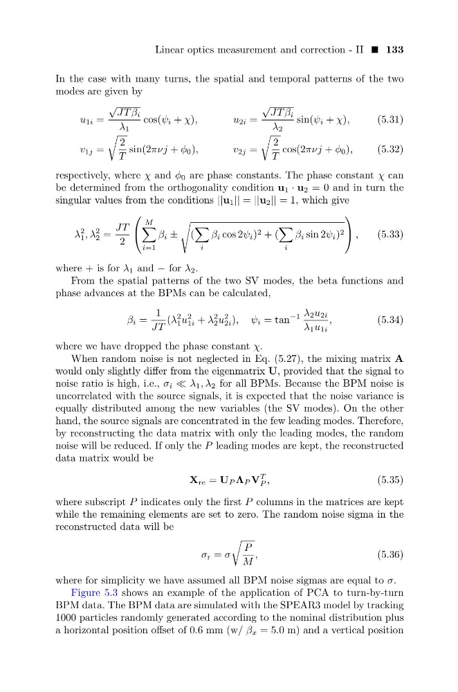
In the case with many turns, the spatial and temporal patterns of the two
modes are given by
u 1i =
√
JT β i
λ 1
cos(ψ i + χ),
u 2i =
√
JT β i
λ 2
sin(ψ i + χ),
(5.31)
v 1j =
2
T
sin(2πνj + φ 0 ),
v 2j =
2
T
cos(2πνj + φ 0 ),
(5.32)
respectively, where χ and φ 0 are phase constants. The phase constant χ can
be determined from the orthogonality condition u 1 · u 2 = 0 and in turn the
singular values from the conditions ||u 1 || = ||u 2 || = 1, which give
λ
2
1 , λ
2
2 =
JT
2
M
i=1
β i ±
(
i
β i cos 2ψ i ) 2 + (
i
β i sin 2ψ i ) 2
,
(5.33)
where + is for λ 1 and − for λ 2 .
From the spatial patterns of the two SV modes, the beta functions and
phase advances at the BPMs can be calculated,
β i =
1
JT
(λ
2
1 u
2
1i + λ
2
2 u
2
2i ), ψ i = tan
−1 λ 2 u 2i
λ 1 u 1i
,
(5.34)
where we have dropped the phase constant χ.
When random noise is not neglected in Eq. (5.27), the mixing matrix A
would only slightly differ from the eigenmatrix U, provided that the signal to
noise ratio is high, i.e., σ i λ 1 , λ 2 for all BPMs. Because the BPM noise is
uncorrelated with the source signals, it is expected that the noise variance is
equally distributed among the new variables (the SV modes). On the other
hand, the source signals are concentrated in the few leading modes. Therefore,
by reconstructing the data matrix with only the leading modes, the random
noise will be reduced. If only the P leading modes are kept, the reconstructed
data matrix would be
X re = U P Λ P V
T
P ,
(5.35)
where subscript P indicates only the first P columns in the matrices are kept
while the remaining elements are set to zero. The random noise sigma in the
reconstructed data will be
σ r = σ
P
M
,
(5.36)
where for simplicity we have assumed all BPM noise sigmas are equal to σ.
Figure 5.3 shows an example of the application of PCA to turn-by-turn
BPM data. The BPM data are simulated with the SPEAR3 model by tracking
1000 particles randomly generated according to the nominal distribution plus
a horizontal position offset of 0.6 mm (w/ β x = 5.0 m) and a vertical position
In the case with many turns, the spatial and temporal patterns of the two
modes are given by
u 1i =
√
JT β i
λ 1
cos(ψ i + χ),
u 2i =
√
JT β i
λ 2
sin(ψ i + χ),
(5.31)
v 1j =
2
T
sin(2πνj + φ 0 ),
v 2j =
2
T
cos(2πνj + φ 0 ),
(5.32)
respectively, where χ and φ 0 are phase constants. The phase constant χ can
be determined from the orthogonality condition u 1 · u 2 = 0 and in turn the
singular values from the conditions ||u 1 || = ||u 2 || = 1, which give
λ
2
1 , λ
2
2 =
JT
2
M
i=1
β i ±
(
i
β i cos 2ψ i ) 2 + (
i
β i sin 2ψ i ) 2
,
(5.33)
where + is for λ 1 and − for λ 2 .
From the spatial patterns of the two SV modes, the beta functions and
phase advances at the BPMs can be calculated,
β i =
1
JT
(λ
2
1 u
2
1i + λ
2
2 u
2
2i ), ψ i = tan
−1 λ 2 u 2i
λ 1 u 1i
,
(5.34)
where we have dropped the phase constant χ.
When random noise is not neglected in Eq. (5.27), the mixing matrix A
would only slightly differ from the eigenmatrix U, provided that the signal to
noise ratio is high, i.e., σ i λ 1 , λ 2 for all BPMs. Because the BPM noise is
uncorrelated with the source signals, it is expected that the noise variance is
equally distributed among the new variables (the SV modes). On the other
hand, the source signals are concentrated in the few leading modes. Therefore,
by reconstructing the data matrix with only the leading modes, the random
noise will be reduced. If only the P leading modes are kept, the reconstructed
data matrix would be
X re = U P Λ P V
T
P ,
(5.35)
where subscript P indicates only the first P columns in the matrices are kept
while the remaining elements are set to zero. The random noise sigma in the
reconstructed data will be
σ r = σ
P
M
,
(5.36)
where for simplicity we have assumed all BPM noise sigmas are equal to σ.
Figure 5.3 shows an example of the application of PCA to turn-by-turn
BPM data. The BPM data are simulated with the SPEAR3 model by tracking
1000 particles randomly generated according to the nominal distribution plus
a horizontal position offset of 0.6 mm (w/ β x = 5.0 m) and a vertical position