

132 Beam-based Correction and Optimization for Accelerators
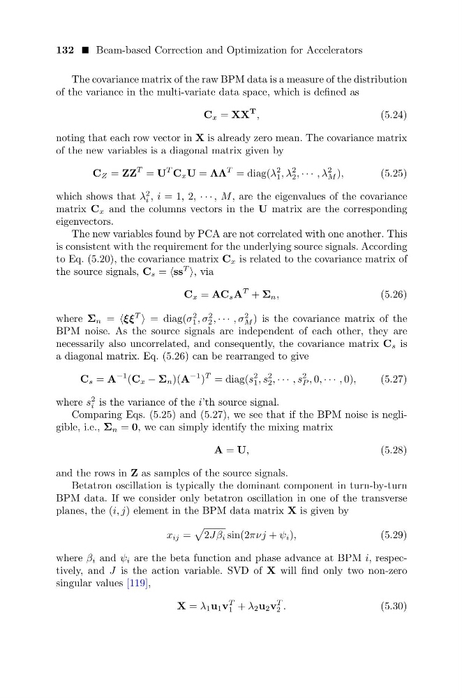
The covariance matrix of the raw BPM data is a measure of the distribution
of the variance in the multi-variate data space, which is defined as
C x = XX
T ,
(5.24)
noting that each row vector in X is already zero mean. The covariance matrix
of the new variables is a diagonal matrix given by
C Z = ZZ
T = U
T C x U = ΛΛ
T = diag(λ
2
1 , λ
2
2 , · · · , λ
2
M ),
(5.25)
which shows that λ
2
i , i = 1, 2, · · · , M , are the eigenvalues of the covariance
matrix C x and the columns vectors in the U matrix are the corresponding
eigenvectors.
The new variables found by PCA are not correlated with one another. This
is consistent with the requirement for the underlying source signals. According
to Eq. (5.20), the covariance matrix C x is related to the covariance matrix of
the source signals, C s = ss
T , via
C x = AC s A
T + Σ n ,
(5.26)
where Σ n = ξξ
T = diag(σ
2
1 , σ
2
2 , · · · , σ
2
M ) is the covariance matrix of the
BPM noise. As the source signals are independent of each other, they are
necessarily also uncorrelated, and consequently, the covariance matrix C s is
a diagonal matrix. Eq. (5.26) can be rearranged to give
C s = A
−1 (C x − Σ n )(A
−1 )
T = diag(s
2
1 , s
2
2 , · · · , s
2
P , 0, · · · , 0),
(5.27)
where s
2
i is the variance of the i’th source signal.
Comparing Eqs. (5.25) and (5.27), we see that if the BPM noise is negligible, i.e., Σ n = 0, we can simply identify the mixing matrix
A = U,
(5.28)
and the rows in Z as samples of the source signals.
Betatron oscillation is typically the dominant component in turn-by-turn
BPM data. If we consider only betatron oscillation in one of the transverse
planes, the (i, j) element in the BPM data matrix X is given by
x ij =
2Jβ i sin(2πνj + ψ i ),
(5.29)
where β i and ψ i are the beta function and phase advance at BPM i, respectively, and J is the action variable. SVD of X will find only two non-zero
singular values [119],
X = λ 1 u 1 v
T
1 + λ 2 u 2 v
T
2 .
(5.30)
The covariance matrix of the raw BPM data is a measure of the distribution
of the variance in the multi-variate data space, which is defined as
C x = XX
T ,
(5.24)
noting that each row vector in X is already zero mean. The covariance matrix
of the new variables is a diagonal matrix given by
C Z = ZZ
T = U
T C x U = ΛΛ
T = diag(λ
2
1 , λ
2
2 , · · · , λ
2
M ),
(5.25)
which shows that λ
2
i , i = 1, 2, · · · , M , are the eigenvalues of the covariance
matrix C x and the columns vectors in the U matrix are the corresponding
eigenvectors.
The new variables found by PCA are not correlated with one another. This
is consistent with the requirement for the underlying source signals. According
to Eq. (5.20), the covariance matrix C x is related to the covariance matrix of
the source signals, C s = ss
T , via
C x = AC s A
T + Σ n ,
(5.26)
where Σ n = ξξ
T = diag(σ
2
1 , σ
2
2 , · · · , σ
2
M ) is the covariance matrix of the
BPM noise. As the source signals are independent of each other, they are
necessarily also uncorrelated, and consequently, the covariance matrix C s is
a diagonal matrix. Eq. (5.26) can be rearranged to give
C s = A
−1 (C x − Σ n )(A
−1 )
T = diag(s
2
1 , s
2
2 , · · · , s
2
P , 0, · · · , 0),
(5.27)
where s
2
i is the variance of the i’th source signal.
Comparing Eqs. (5.25) and (5.27), we see that if the BPM noise is negligible, i.e., Σ n = 0, we can simply identify the mixing matrix
A = U,
(5.28)
and the rows in Z as samples of the source signals.
Betatron oscillation is typically the dominant component in turn-by-turn
BPM data. If we consider only betatron oscillation in one of the transverse
planes, the (i, j) element in the BPM data matrix X is given by
x ij =
2Jβ i sin(2πνj + ψ i ),
(5.29)
where β i and ψ i are the beta function and phase advance at BPM i, respectively, and J is the action variable. SVD of X will find only two non-zero
singular values [119],
X = λ 1 u 1 v
T
1 + λ 2 u 2 v
T
2 .
(5.30)