

Linear optics measurement and correction - I 119
0
50
100
150
200
s (m)
0.6
0.8
1
1.2
1.4
x
/
x
before
after
0
50
100
150
200
s (m)
0.8
0.9
1
1.1
1.2
y
/
y
before
after
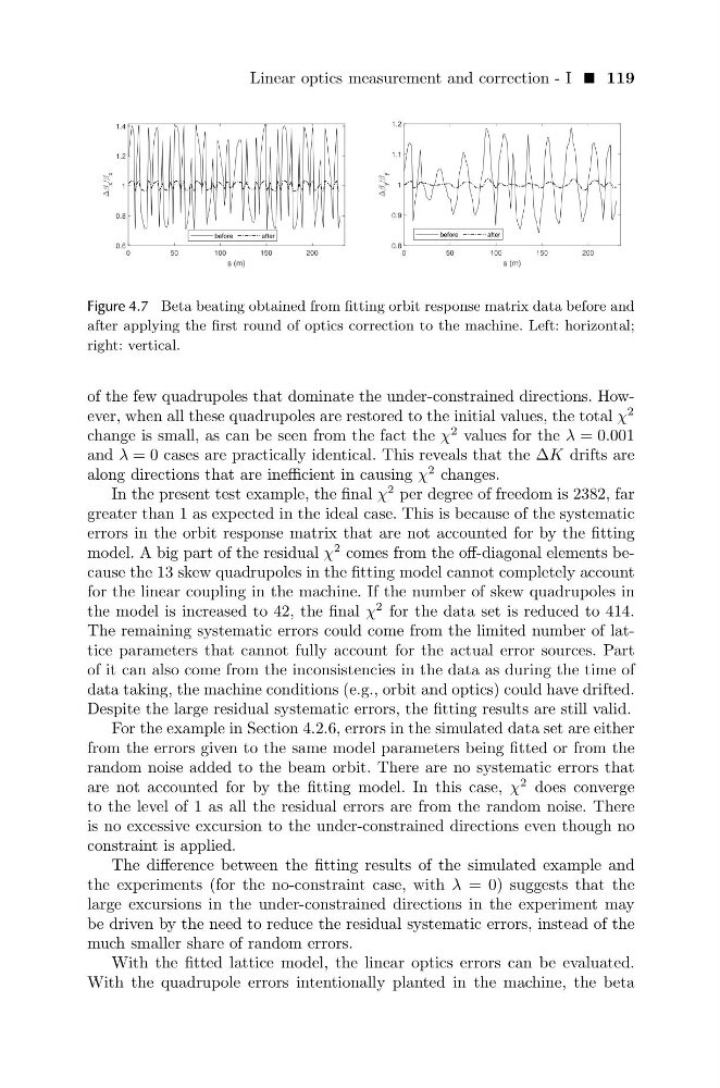
Figure 4.7 Beta beating obtained from fitting orbit response matrix data before and
after applying the first round of optics correction to the machine. Left: horizontal;
right: vertical.
of the few quadrupoles that dominate the under-constrained directions. However, when all these quadrupoles are restored to the initial values, the total χ
2
change is small, as can be seen from the fact the χ
2 values for the λ = 0.001
and λ = 0 cases are practically identical. This reveals that the ∆K drifts are
along directions that are inefficient in causing χ
2 changes.
In the present test example, the final χ
2 per degree of freedom is 2382, far
greater than 1 as expected in the ideal case. This is because of the systematic
errors in the orbit response matrix that are not accounted for by the fitting
model. A big part of the residual χ
2 comes from the off-diagonal elements because the 13 skew quadrupoles in the fitting model cannot completely account
for the linear coupling in the machine. If the number of skew quadrupoles in
the model is increased to 42, the final χ
2 for the data set is reduced to 414.
The remaining systematic errors could come from the limited number of lattice parameters that cannot fully account for the actual error sources. Part
of it can also come from the inconsistencies in the data as during the time of
data taking, the machine conditions (e.g., orbit and optics) could have drifted.
Despite the large residual systematic errors, the fitting results are still valid.
For the example in Section 4.2.6, errors in the simulated data set are either
from the errors given to the same model parameters being fitted or from the
random noise added to the beam orbit. There are no systematic errors that
are not accounted for by the fitting model. In this case, χ
2 does converge
to the level of 1 as all the residual errors are from the random noise. There
is no excessive excursion to the under-constrained directions even though no
constraint is applied.
The difference between the fitting results of the simulated example and
the experiments (for the no-constraint case, with λ = 0) suggests that the
large excursions in the under-constrained directions in the experiment may
be driven by the need to reduce the residual systematic errors, instead of the
much smaller share of random errors.
With the fitted lattice model, the linear optics errors can be evaluated.
With the quadrupole errors intentionally planted in the machine, the beta
0
50
100
150
200
s (m)
0.6
0.8
1
1.2
1.4
x
/
x
before
after
0
50
100
150
200
s (m)
0.8
0.9
1
1.1
1.2
y
/
y
before
after
Figure 4.7 Beta beating obtained from fitting orbit response matrix data before and
after applying the first round of optics correction to the machine. Left: horizontal;
right: vertical.
of the few quadrupoles that dominate the under-constrained directions. However, when all these quadrupoles are restored to the initial values, the total χ
2
change is small, as can be seen from the fact the χ
2 values for the λ = 0.001
and λ = 0 cases are practically identical. This reveals that the ∆K drifts are
along directions that are inefficient in causing χ
2 changes.
In the present test example, the final χ
2 per degree of freedom is 2382, far
greater than 1 as expected in the ideal case. This is because of the systematic
errors in the orbit response matrix that are not accounted for by the fitting
model. A big part of the residual χ
2 comes from the off-diagonal elements because the 13 skew quadrupoles in the fitting model cannot completely account
for the linear coupling in the machine. If the number of skew quadrupoles in
the model is increased to 42, the final χ
2 for the data set is reduced to 414.
The remaining systematic errors could come from the limited number of lattice parameters that cannot fully account for the actual error sources. Part
of it can also come from the inconsistencies in the data as during the time of
data taking, the machine conditions (e.g., orbit and optics) could have drifted.
Despite the large residual systematic errors, the fitting results are still valid.
For the example in Section 4.2.6, errors in the simulated data set are either
from the errors given to the same model parameters being fitted or from the
random noise added to the beam orbit. There are no systematic errors that
are not accounted for by the fitting model. In this case, χ
2 does converge
to the level of 1 as all the residual errors are from the random noise. There
is no excessive excursion to the under-constrained directions even though no
constraint is applied.
The difference between the fitting results of the simulated example and
the experiments (for the no-constraint case, with λ = 0) suggests that the
large excursions in the under-constrained directions in the experiment may
be driven by the need to reduce the residual systematic errors, instead of the
much smaller share of random errors.
With the fitted lattice model, the linear optics errors can be evaluated.
With the quadrupole errors intentionally planted in the machine, the beta